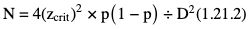
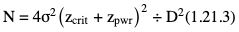
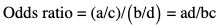
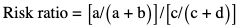
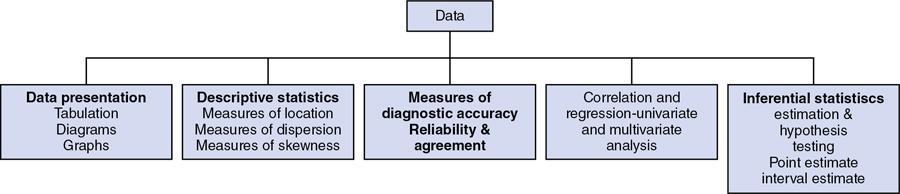
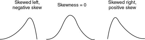
Amarnath C, Arun Murugan, Sam Kamelsen, Rajashree R Statistics is the Grammar of Science. Karl Pearson The goal of any clinical research is to improve patient care. The performance and publication of research and studies evaluate the utility of imaging modalities and their applications. These are important for directing clinical recommendations and developing practice guidelines. Biostatistics is defined as the application of statistical principles and techniques to biological, medical and public health research. Knowledge of biostatistical concepts will help the practicing radiologist to conduct scientifically rigorous studies and to critically evaluate the literature and to make informed clinical decisions. Exposure to research methodology, in general and statistics in particular, is limited over the course of radiology training. The clinical workload of radiologists, limited resources on research methods tailored for radiologists and the lack of interest to learn greatly hinder development of these skills. Poor knowledge of biostatistics and its inappropriate application can lead to studies with incorrect results and potentially wrong clinical implications. This chapter is an effort to prime the radiologists regarding research methodology with a focus on biostatistics. Guidelines for manuscript writing are discussed in Chapter 1.31. A good study design forms the foundation for a research from which clinical implications can be made. A poorly performed statistical analysis can even be repeated, whereas a carelessly done study cannot be redeemed. The steps in planning and execution of a study/research include (Table 1.21.1): Research topic Review of literature Research question Research hypothesis Research Design Data collection Data processing and presentation Data analysis Data interpretation Discussion A detailed checklist for Strengthening the Reporting of Observational Studies in Epidemiology (STROBE) statement is enclosed in the annexure. Research studies can be broadly classified as Observational and experimental, based on whether the investigator assigns the exposure/intervention (Fig. 1.21.1). Preclinical imaging trials involve the visualization of living animals for research purposes, such as disease models and drug development. Imaging modalities help in observing changes, either at the molecular, cell, tissue or organ level in animals responding to physiological or pathological stimuli. Imaging modalities have an advantage of being non-invasive and in vivo. They can be broadly classified into anatomical and functional imaging techniques. Anatomical imaging is done using ultrasound, magnetic resonance imaging and computed tomography. Whereas optical imaging, perfusion and other functional cross-sectional imaging, positron emission tomography (PET) and single photon emission computed tomography (SPECT) are usually used for functional imaging. Clinical Trials are experimental studies used for the introduction of a new intervention, conventionally a new drug, but can also be extended to include trials used for the evaluation of a new stent or type of coil for embolization. They consist of four phases (Table 1.21.3). Example: Comparison of uterine artery embolization and high intensity focussed ultrasound for the management of uterine fundal leiomyomas. Multi-centric study: A multi-centric study is a study that is conducted at more than one research or medical centre. The advantages include a large number of geographically varied subjects and the ability to compare results from all of these groups. The most common disadvantage of randomized clinical trials is their high expense. Hence, multi-centric trials that utilize cooperation between many research centres are becoming more common. For example, MDCT characterization of the Severe Acute Respiratory Syndrome coronavirus 2(SARS-CoV-2) pneumonia has been done as a multi-centric trial in order to obtain and analyze information on the pathogenesis of this novel infectious disease across geographic boundaries. Reviews are vital instruments for researchers and clinicians who want to be up to date with the evidence that has been accumulated in their fields. They can be structured-systematic reviews, meta-analysis and pooled analysis or unstructured-narrative reviews/commentary. The structured reviews enable evaluation of existing evidence on a topic of interest and concludes to confirm/support a practice, refute a practice or identify areas for which additional investigations are needed. A systematic review involves selecting, assessing and synthesizing all available data. Whereas meta-analysis employs statistical methods in combining the evidence/data derived from a systematic-review of multiple studies that aim to address the same clinical and scientific question. For example, MRI for Detecting Root Avulsions in Traumatic Adult Brachial Plexus Injuries: A Systematic Review and Meta-Analysis of Diagnostic Accuracy Ryckie G. Wade et al. 11 studies of 275 adults (mean age, 27 years; 229 men) performed between 1992 and 2016 were included for analysis. The initial steps in planning a study include PICO (Population, Intervention, Control group and Outcome) is a useful acronym for formulating a research question for various study designs (Table 1.21.4). Characteristics of a good research question can be summarized using the acronym (FINER): Feasible-adequacy of sample, affordability in time and money, I: Interesting-getting the answer excites the investigator, peers, community, N: Novel-confirms/refutes/extends previous findings, E: Ethical-beneficial without causing harm and in accordance with ethical principles, R: Relevant to advance scientific knowledge, health policy, to enable future research. Table 1.21.5 presents study designs with research questions formulated using PICO approach. Reproduced from D. Sackett, W.S. Richardson, W. Rosenburg, R.B. Haynes. How to practice and teach evidence based medicine, second ed., Churchill Livingstone, 1997. “Is ultrasound (index test) as accurate as MRI (reference standard) to determine the position of the placenta in pregnant women with clinically suspected placenta previa?” Pregnant women with clinically suspected placenta previa “Is Gadobenate Dimeglumine able to cause nephrogenic systemic fibrosis in patients with chronic kidney disease?” Patients with chronic kidney disease “Is fetal MRI performed during the third trimester of gestation able to cause learning disability in this population by the time they reach school age?” Children of school age who underwent a fetal MRI in their third trimester of gestation “Does hormone replacement therapy increase the risk of having a mammographic density?” Patients with mammographic density “Does the use of radiofrequency ablation for solitary unresectable hepatocellular carcinoma result in better outcome compared to trans-arterial chemoembolization?” Experimental intervention: Radiofrequency ablation Standard intervention: Trans-arterial chemoembolization A sample is a group of individuals who are the study subjects and should be representative of the entire population. As one cannot practically study the entire population, sampling is done. Sampling should be done in such a manner that the results can be generalized to the entire population. Samples can be drawn from the entire population through various methods, broadly classified into two groups (Fig. 1.21.2). Every individual has an equal chance of being selected for the study in simple random sampling. Usually a computer-created list of random numbers is used to select a simple random sample. A systematic random sample is one in which every nth item is selected. For example, every fifth patient scanned is included in a study. In stratified random sampling, the population is first divided into subgroups and then sampled. A cluster sample is used more often in epidemiologic research than in clinical studies. Both random samples and randomization involve the use of the probability sampling method, but are different concepts (Table 1.21.6). Sample Size: It is vital to design studies with the suitable prospect of detecting effects when they are really present, and not sensing effects when they are not. Statistical power is the probability that a statistical test will indicate a significant difference when there truly is one. Statistical power is in turn determined by sample size. The sample size must be large enough for the study to have appropriate statistical power. A number of study design factors influence the calculation of sample size, like prevalence of the disease, the minimum expected difference between the two means and acceptable error. There are many formulae and computer applications that simplify the task considerably. In studies designed to estimate a mean, the equation for sample size is: N = 4 σ 2 ( z crit ) 2 ÷ D 2 (Eq. 1.21.1) where Example, suppose a radiologist wants to determine the mean fetal biparietal diameter in a group of patients in the second trimester of pregnancy. The required limits of the 95% confidence interval is mean biparietal diameter ±1 mm. From existing studies, it is known that the SD for the measurement is 4 mm. Based on these assumptions, D = 2 mm, σ = 4 mm, and zcrit = 1.960 (for 95% CI). N = 4 × (4)2 × (1.96)2/4 = 4 × 16 × 3.84/4 = 61.4. Eq. (1.21.1) yields a sample size of N = 61. Therefore, 61 fetuses should be examined in the study. In studies where the scale of measurement is in terms of a proportion, the equation for sample size is given by Eq. (1.21.2) N = 4 ( z crit ) 2 × p ( 1 − p ) ÷ D 2 (1.21.2) where p is a pre-study estimate of the proportion to be measured, and N, zcrit and D are defined as they are for Eq. (1.21.1). For example, suppose an investigator would like to determine the accuracy of a diagnostic test with a 95% CI of ±10%. Consider that on the basis of results of earlier studies, the estimated accuracy is 80%. With these assumptions, D = 0.20, P = .80 and zcrit = 1.960. N = 4 × ( 1.96 ) 2 × 0.8 ( 1 − 0.8 ) / 0.04 = 4 × 3 . 84 × 0 . 8 × 0 . 2 / 0 . 04 = 61 . 4 Eq. (1.21.2) yields a sample size of N = 61. Therefore, 61 patients should be examined in the study. Sample size estimation for comparative studies. For a study in which two means are compared, sample size can be determined using Eq. (1.21.3) N = 4 σ 2 ( z crit + z pwr ) 2 ÷ D 2 (1.21.3) where Example: Consider a study planned to compare renal artery stenting versus medical therapy in lowering the mean blood pressure of patients with secondary hypertension due to renal artery stenosis. Based on existing literature, the investigators estimate that renal artery stenting may help lower blood pressure by 20 mm Hg, while medical therapy may help lower blood pressure by only 10 mm Hg. Based on existing literature, the standard deviation (SD) for lowering blood pressure is estimated to be 20 mm Hg. According to the normal distribution, this SD indicates an expectation that 95% of the patients in either group will experience a blood pressure lowering within 40 mm Hg (2 SDs) of the mean. A significance criterion of.05 and power of 0.80 are chosen. With these assumptions, D = 20 – 10 = 10 mm Hg, σ = 20 mm Hg, zcrit = 1.960, and z = 0.842. N = 4 × (20)2 × (1.96 + 0.842)2/102 = 4 × 400 × (2.802)2/100. = 1600 × 7.85/100 = 125.6. Eq. (1.21.3) yields a sample size of N∼126. Therefore, a total of 126 patients should be enroled in the study: 63 to undergo renal artery stenting and 63 to receive medical therapy. For a study in which two proportions are compared with Chi square test, the equation for sample size estimation is Eq. (1.21.4) N = 2 [ z crit 2P ¯ ( 1 − P ¯ ) + z pwr ( P 1 ( 1 − P1 ) + P2 ( 1 − P2 ) ) ] 2 ÷ D 2 (1.21.4) where P1 and P2 denote pre-study estimates of the two proportions to be compared, the minimum expected difference, D = P1 – P2. Assumptions of this calculation include equal samples of N in the two groups and that two-tailed statistical analysis will be used. It is to be noted that in this case, N depends on the magnitude of the two proportions in addition to their difference. Hence, Eq. (1.21.4) requires the estimation of P1 and P2, as well as their difference, before performance of the study. However, Eq. (1.21.4) does not require a separate estimate of standard deviation because it is calculated within the equation using P1 and P2. Example, suppose USG has an accuracy of 80% for the diagnosis of focal liver lesions. A study is proposed to evaluate contrast-enhanced USG that may have greater accuracy. On the basis of their experience, the investigators decide that contrast-enhanced USG would have to be at least 90% accurate to be considered significantly better than the standard USG. A significance criterion of.05 and a power of 0.90 are chosen. With these assumptions, P1 = 0.80, P2 = 0.90, D = 0.10, Eq. (1.21.2) yields a sample size of N = 398. Therefore, a total of 398 patients should be enroled: 199 to undergo USG and 199 to undergo contrast-enhanced USG. Bias is persistent non-random error. Unlike random error, bias is systematic. For example, an inaccurately standardized CT scanner that gives CT attenuation values of +10 HU greater than the actual values for all tissues. Bias reduces the accuracy of study results and is not affected by a change in the size of the sample. Source of bias are multiple, right from selection of sample, performance of the diagnostic test/reference standard, interpretation of test result and analyzing the results. This makes it very difficult to design and interpret studies. Researchers should implement ways to circumvent bias or to minimize its effect while still in the initial phase of planning. Some common bias encountered include, but not limited to, the following: Confounder is a factor that is associated with both the outcome and the exposure. Confounders change or distort real associations between the exposure and outcome variables. Example: consider a study done to assess if alcohol use (exposure) is related to increased incidence of lung cancer. It may be confounded by the effects of smoking which is associated with both the exposure and the outcome. Confounding can be reduced by measures such as matching and stratified analysis. Effect modifiers are associated with the outcome but not the exposure. For example, in a study to assess association of thorotrast (exposure) with hepatic malignancy (outcome), Hepatitis B viral infection may be considered an effect modifier as it is associated with the outcome but not the exposure factor. Rate is a ratio where the denominator is in units of time, e.g. mortality rate. Rates and proportions are ratios, though not synonyms. Ratio is the value obtained by dividing one quantity by another, e.g. ratio of male to female patients visiting USG OPD, signal to noise ratio. Proportion is a ratio where the numerator is included in the population defined by the denominator. It may be used for measured data as well as count/frequency. As the numerator is part of the denominator, it has no dimension. However, it can be expressed as a percentage, e.g. Proportion of male patients is obtained by dividing the male patients by the total number of patients; Proportion of patients with a positive diagnosis, proportion of lung area affected in CT. Incidence is the number of new patients per unit of time (usually per year). It is a rate. Prevalence is the total number of existing patients in a population at a point of time. It is a proportion. Prevalence of a disease = Incidence rate × average duration of the disease Odds is the ratio of the probability of occurrence of an event to that of nonoccurrence, or the ratio of the probability that something is one way to the probability that it is another way. Odds = probability/1 − probability. Consider the hypothetical situation: If 60 out of 100 interventional radiologists develop a cataract and remaining 40 don’t develop cataract, the odds in favour of developing a cataract are 60 to 40, or 1.5; this is different from the risk that they will develop a cataract, which is 60 over 100 or 0.6. Odds ratio is the ratio between two odds. Odds ratio = ( a/c ) / ( b/d ) = ad / bc The exposure-odds ratio for data obtained from cross-sectional or case–control studies is the ratio of the odds in favour of exposure among the cases (a/b) to the odds in favour of exposure among controls (c/d). This can be simplified as ad/bc (Table 1.21.7). The odds ratio obtained in a case–control study accurately estimates risk ratio when the outcome in the population being studied is rare. The relative risk (also called the risk ratio) is the ratio of the risk of occurrence of a disease among exposed people to that among the unexposed. Table 1.21.8 demonstrates tabulation of data in a cohort study to obtain the relative risk. Risk ratio = [ a / ( a + b ) ] / [ c / ( c + d ) ] The risk ratio (RR) provides an estimate of the strength of association between the exposure and outcome. RR > 1 indicates positive association between outcome and exposure, RR > 1 indicates positive association between outcome and exposure, RR < 1 indicates that a given exposure is associated with a decreased risk of the outcome. RR = 1 indicates that a given exposure is not associated with a risk of the outcome. Attributable risk is the rate of an outcome in exposed individuals that can be attributed to the exposure. This is a more useful from a public health perspective. Association and causation: An association is a measurable change in one variable that occurs simultaneously with changes in another variable. Statistical methods establish evidence of a relationship between exposure and outcome, which must be validated by clinical judgement and reasoning of the study in order to establish causation. Causation includes the elements of precedence, non-spuriousness and plausibility in addition to a strong association between the variables in question. A variable is a measure whose value can vary, e.g. age, gender, weight, liver size, vessel diameter, etc. The values of these variables can change from one individual to another. A dependent/outcome variable depends on variations in another variable. An independent/predictor variable can be manipulated to affect variations or responses in another variable. Covariates are independent variables that function along with predictors to influence outcomes and might be confounders and hence should be taken into account during the planning phase of the study. Data are simply a collection of variables. Data and descriptive statistics form the building blocks for inferential statistics and are essential for choosing appropriate advanced analytical methods. Descriptive statistics provides cursory insight on almost any type of data and helps identify patterns which lead to generation of hypothesis. Unorganized data are known as raw data. The data collected in studies can be very voluminous and be difficult to comprehend. In order to be meaningful and for further analysis, data have to be summarized using certain tools such as tables, graphs and measures of central tendency and dispersion as appropriate. This process of summarizing data is known as descriptive statistics. The data collected from studies can be analyzed further as depicted in Fig. 1.21.3. Data collected from studies can be classified into two types: Quantitative data and qualitative data. Qualitative/Categorical data can be classified further as nominal, binary, ordinal. Quantitative data can be classified as discrete or continuous (Table 1.21.9). Mode – Mode – Median Inter-quartile range Symmetrical-mean Skewed-median Standard deviation Inter-quartile Range Symmetrical-mean Skewed-median Standard deviation Quartile Range Interval scale and Ratio scale are alternative classification of Quantitative data. Interval scale: On an interval scale, the quantitative values have an order and there is meaningful difference between the variables. However, there is no clearly defined zero which is arbitrary. Ratio scale: It is similar to interval scale and, in addition, has a clearly defined zero. For example, temperature is not ratio data because one temperature cannot be twice as hot as another. If the distribution of the data is normal, the data is described by calculating the mean and SD. Mean and standard deviation are pointless in describing qualitative (categorical) data as they not have meaningful numeric values. Qualitative data are usually described by using proportions and are summarized by frequency (in percentage). The measure of central tendency used for categorical data is the mode. Numerical data has specific numbered values and may be classified as continuous or discrete variables. Continuous data can take all possible numerical value, e.g. weight can be 45, 45.1, 45.2, etc., whereas discrete variables are usually whole numbers. The same data can be measured using different scales. For example, The NASCET criteria (North American Symptomatic Carotid Endarterectomy Trial, 1991) commonly used for the classification of carotid artery stenosis has the following categories: less than 30% denotes mild stenosis; 30%–69% indicates moderate stenosis; greater than 70% denotes severe stenosis. Here percentage of occlusion, which is a continuous variable, is converted into three categories (i.e. ordinal data) – a different scale of measurement. Visual representation of data can be done using graphs/charts (Table 1.21.10), which can be classified into the following four categories based on their specific purpose: Used to depict comparison between categories of data, the gaps indicate that the data is categorical or discrete. The error bars are measures of uncertainty and may represent standard deviation/confidence interval or standard error – they should not be used to draw conclusions. Used to represent multiple categories of data, e.g. male and female patients with varying grades of disease. They can also be used to denote multiple categories. Similar to a bar chart, but there are no gaps between the bars as the data is continuous. It is helpful in analyzing distribution of the data – whether normal distribution or not. Helps in visualization of the trends in data over intervals of time, e.g. number of monthly MRI examinations in a year. Box-and-whisker plots consist of a box with a horizontal dividing line representing the median. The top of the box represents the 75th percentile, bottom the 25th percentile (the first and third quartiles). The box represents the interquartile range. The range of values and outliers are also represented. Points show the relationship between two sets of continuous data. Used to represent numerical proportions of categorical data. The quantitative estimation for each category is proportional to the angle made at the centre of the circle and thus to the area of the sector. A forest plot is a plot used to represent the list of studies in the systematic review. The outcome of multiple studies are represented on the vertical axis and the outcome measure on the horizontal axis. The outcome measure might be odds or risk ratios. The data may be displayed by using a box-shape whose position represents the point estimate, with a horizontal line through it whose length represents the width of the 95% confidence interval for whatever outcome measure is being used. The area of each box is proportional to its sample size/power. The diamond at the bottom represents the combined result. If it does not cross the vertical line of no effect, then the study is statistically significant. Other descriptive methods/measures include frequency distribution is a table that shows a body of data grouped according to numeric values. Frequency polygon is a graphic method of presenting a frequency distribution. Range: It is the difference between the largest and smallest values. It is a measure of dispersion. Percentile: Data points that cut the data into 100 segments. Quartile represents 25% of data and interquartile range (IQR) is the measure of dispersion that is equal to the difference between the 75th and 25th percentiles. IQR = Q3 – Q1. A distribution is a representation of the frequencies of the values of a measurement obtained from specified groups. Out of all the possible values that the measurement can have, the distribution tells what proportion of the group was found to have each value (or each range of values). Distributions have certain properties as depicted in Table 1.21.12. Mean = sum of values/total number of values-most affected by outliers (extreme values) Population mean is represented by µ Sample mean is represented by Mean = 121/11 = 11 Standard deviation (SD, σ) denotes variability in a set of values around the mean of the set. It is a range n = The number of date points xi = Each of the values of the data An asymmetric distribution also called a skewed distribution. The tail of the distribution determines the direction of skewness – tail to the right indicates positive skew, tail to the left indicates negative skew (Fig. 1.21.12) Median = middle value of a sorted list from least to greatest value Variance – square of the standard deviation Kurtosis It is the extent to which a unimodal distribution is peaked Mode = most repeated value. Standard error – an estimate of variability that exists in a set of sample means around the true population mean Standard error of the sample means SE (mean) = The normal distribution (Fig. 1.21.13) commonly describes clinical data, and is symmetrical and bell-shaped, with mean, median and mode equal to each other. It is also called a Gaussian distribution. About two-thirds of the values under a normal distribution curve fall within one standard deviation (SD) of the mean, and approximately 95% fall within two standard deviations of the mean. Normal Distributions have tails which get closer to the horizontal axis, but never touch it. It takes two parameters to specify an individual: Normal Distribution – the Mean, μ, and the Standard Deviation, σ. The Standard Normal Distribution (whose Test Statistic is z) has μ = 0 and σ = 1. There is an empirical rule that the cumulative probabilities bounded by standard deviations are the same for all normal distributions – roughly 68%, 95% and 99.7% for 1, 2 and 3 standard deviations, respectively. Normal Distributions are by far the most common type of distribution one encounters in statistics and in our daily lives. They are common in natural and human physiological processes that are influenced by many small and unrelated random effects. Some examples include height or weight of individuals of the same gender, test scores and blood pressure. Other distributions include binomial, t-distribution, chi-square, Poisson, exponential, lognormal, uniform distribution, etc. Properties of Diagnostic Tests: Diagnostic studies examine the ability of diagnostic tests to discriminate correctly between patients with and without particular medical conditions. Properties of a diagnostic test can be broadly classified under two categories: The ideal diagnostic test should be accurate as well as precise (Fig. 1.21.14A). Reliability and validity can be illustrated by the four scenarios using a target. The centre of the target denotes the true value and the stars represent the measurements being tested. Scenario (a) shows a measurement that is accurate and precise, (b) shows a measurement that is precise but inaccurate; scenario (c) shows a measurement that is accurate but imprecise and (d) shows a measurement that is both inaccurate and imprecise. Validity, also called accuracy, is the ability of a test to correctly identify patients with the disease and those without the disease (Table 1.21.16). Face validity evaluates whether the test appears to measure the concept. As an example, an MR study of the abdomen will not facilitate a diagnosis for seizure. Predictive validity refers to the ability of a test to correctly predict (or correlate with) an outcome (e.g. an infiltrative lesion and malignancy on subsequent histopathology). Content validity is the extent to which the indicator reflects the full area of interest (e.g. extra-dural haemorrhage resolution might be indicated by haemorrhage height, width or both). Construct validity is the extent to which one measure correlates with other measures of the same concept (e.g. correlation of positive MR study for demyelination with clinical findings). Disease status is usually determined by a reference standard, which is expected to be the best existing measure for determining accurate disease status. Usually tissue diagnosis or an invasive investigation such as angiography are reference standards. Diagnostic accuracy is determined by comparing the test results to the appropriate reference standard. Sensitivity and specificity are intrinsic measures of diagnostic accuracy, i.e. they are not affected by prevalence of the disease. However, disease factors, like the grade of severity, anatomic features (e.g. smaller lesions are less likely to be detectable by imaging) and patient factors (e.g. the efficacy of transabdominal USG in evaluating uterine and adnexal lesions is influenced by the degree of bladder filling) influence the sensitivity and specificity. For this reason, the sensitivity and specificity of individual diagnostic tests should not be considered absolute and should be considered in light of both factors. Example: The sensitivity (95% Confidence Interval within brackets) of ultrasonography (USG) for the diagnosis of appendicitis in children is 85% (82%, 90%). That is, the ability of the USG to classify children as positive when the child really has appendicitis is about 85% on average. Similarly, the specificity is 94% (92%, 96%). That is, the ability of the USG to identify children as negative when the child does not have appendicitis is about 94% on average. Sensitivity and specificity estimation can be performed for tests with ordinal or continuous results, only after a decision threshold (termed a cut-off point). A cut-off is necessary to separate positive from negative results. For example, a mammogram may be interpreted as normal, benign, probably benign, suspicious or malignant. A positive test result may be defined anywhere along this spectrum, other than normal. A cut-off is decided by the research context. A screening test will have threshold values set for more sensitivity (a higher decision threshold), while a confirmatory/diagnostic test will have cut-offs set for more specificity (a lower decision threshold). The sensitivity and specificity of a diagnostic test with binary (positive or negative) results are represented by a 2 × 2 contingency table, where columns show test results and the rows show the disease status. The disease status may be assessed using a reference standard. The table has four cells:
1.21: Research methodology and biostatistics
RESEARCH DESIGN
Planning
Execution
Study types
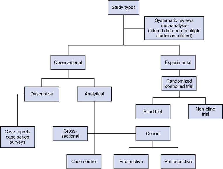
Experimental study
Phase
Population
Purpose
Phase 1
Healthy volunteers
Document the safety of the intervention in humans
Phase 2
Small group of real patients
Focus on efficacy while still providing information on safety
Phase 3
Randomized controlled trials involving large group of real patients
Efficacy of different modes of administration of the intervention to patients
Phase 4
Post-marketing studies of the intervention
Possible long-term adverse events not yet documented
Systematic reviews and meta-analysis
Planning a study
Research question
Population
Who is the study population?
Intervention
What is the intervention/diagnostic test of interest?
Control or comparison
What is the intervention/diagnostic test for comparison?
Outcome
What is the outcome of interest?
Population/Cases
Intervention/Exposure
Control
Outcome
Design
None
None
Position of placenta-whether placenta previa
Cross sectional
Gadobenate Dimeglumine
None
Nephrogenic systemic fibrosis
Prospective cohort
Fetal MRI performed during the third trimester of gestation
None
Learning disability at school age
Retrospective cohort
Risk factor: Hormone replacement therapy
Age/sex matched persons without mammographic density
Mammographic density
Case control
Primary endpoint (outcome): Shrinkage of tumour size after 3 months
Patients with unresectable hepatocellular carcinoma are randomized to (i) radiofrequency ablation or (ii) trans-arterial chemoembolization treatment groups
Randomized trials
Sampling techniques

Random Sampling
Randomization
Random sampling determines which individual will be included in the sample.
Randomization, or random assignment, states which subjects to be assigned to the treatment or control group.
It is related to sampling and external validity.
It is related to design and internal validity.
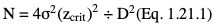
Sample size estimation for descriptive studies


 = (P1 + P2)/2, and N, zcrit and zpwr are as previously defined.
 = (P1+P2)/2
= 0.85, zcrit = 1.960, and zpwr = 0.842.
Potential errors in studies
Basic terms and definitions used in biostatistics
Group
Cases
Controls
Exposed
a
b
Unexposed
c
d
Data and descriptive statistics
Data/ Variable Type
Examples
Best Measure of Central Tendency
Best Measure of Dispersion
Qualitative
Nominal
More than two categories without meaningful order such as an imaging modality (US, CT, MR), ethnicity, months in a year, days of the week, etc.
Dichotomous/Binary
Only two categories such as a disease being present/absent
Ordinal
More than two categories with logical order, e.g. TNM tumour staging, USG echogenicity (anechoic, hypoechoic, hyperechoic), BI-RADS® score system, grading severity as mild, moderate and severe, Arnold–Hilgartner radiographic scale for assessment of severity of haemophilic arthropathy
Quantitative
Discrete
Can take only a limited number of values. Usually involves countNumber of CT scans performed in 1 year, number of liver lesions
Continuous
Can take unlimited number of values, e.g. lesion size, organ volume, artery diameter, Signal to noise ratio (SNR), CT dose, time duration
Descriptive statistics – displaying statistical data
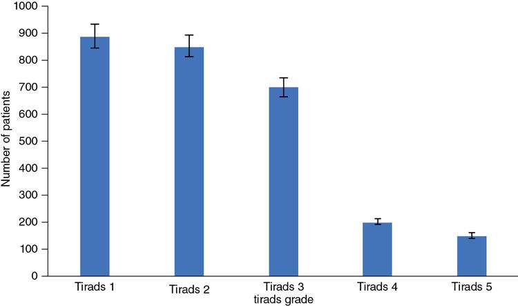
Bar chart
Fig. 1.21.4
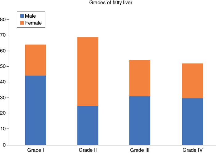
Clustered/stacked bar chart
Fig. 1.21.5
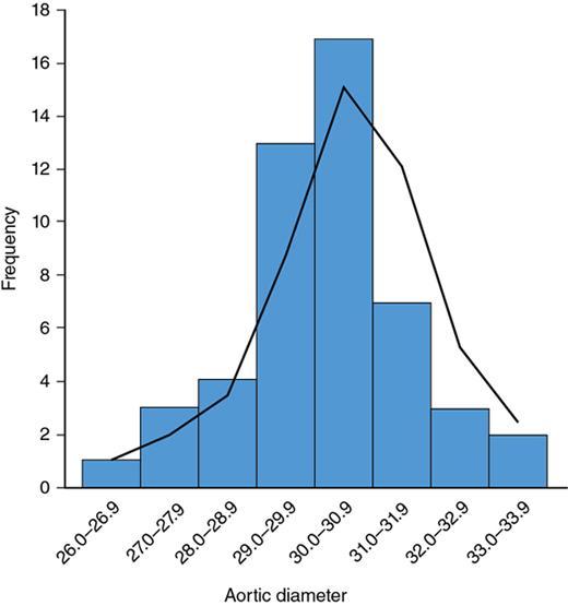
Frequency table of aortic diameters in adults 20–40 years.
Table 1.21.11
Histogram
Fig. 1.21.6
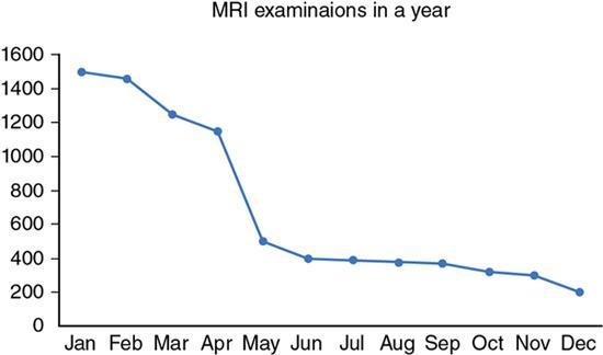
Line diagram
Fig. 1.21.7
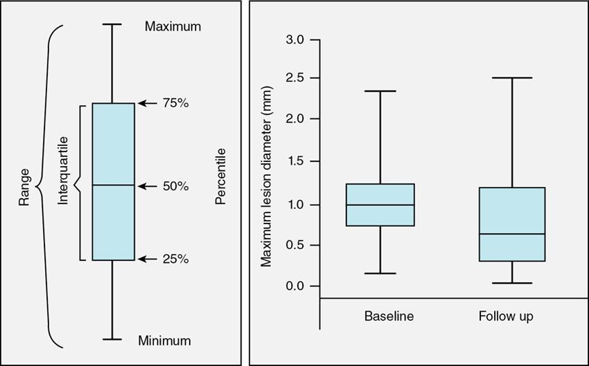
Box and Whisker plot
Fig. 1.21.8
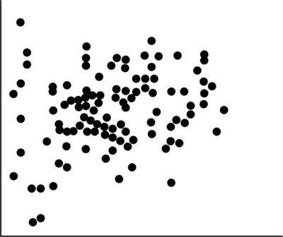
Scatter diagram
Fig. 1.21.9
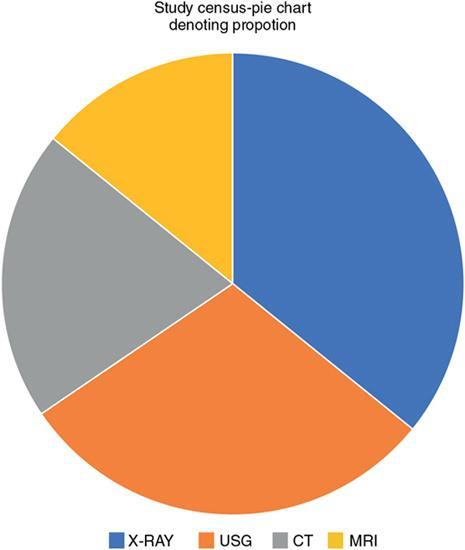
Pie chart
Fig. 1.21.10
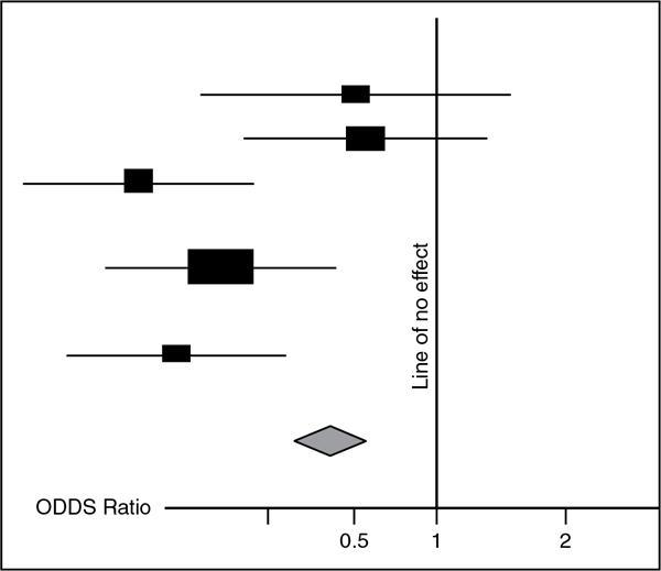
Forest Plot
Fig. 1.21.11
Aortic Diameter (Frequency)
Number of People
26.0–26.9
1
27.0–27.9
3
28.0–28.9
4
29.0–29.9
13
30.0–30.9
17
31.0–31.9
7
32.0–32.9
3
33.0–33.9
2
Distributions
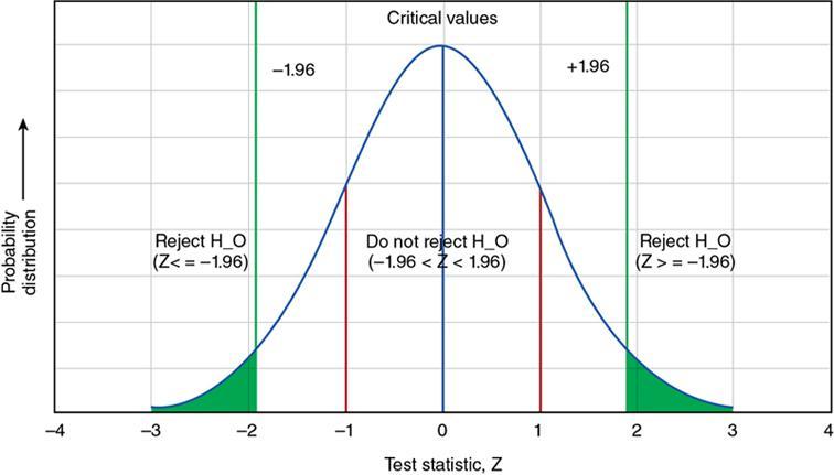
Normal distribution
Measures of Central Tendency
Measures of Dispersion (to what degree are the observations spread or dispersed)
Shape of the Distribution
 , e.g. consider a set of CT attenuation values: 4, 5, 6, 7, 8, 10, 13, 13, 15, 17, 23
 = The mean of the xi

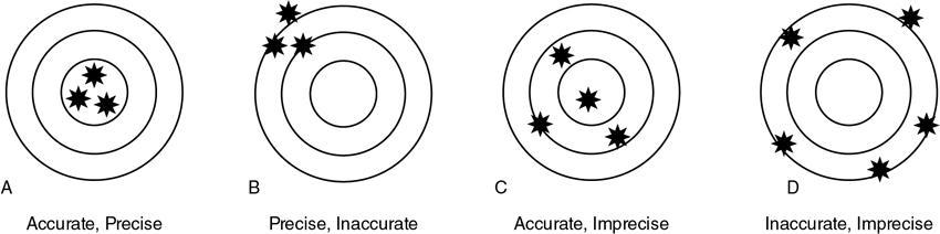
Accuracy/validity
Related posts:

Stay updated, free articles. Join our Telegram channel

Full access? Get Clinical Tree


