Fig. 1
An early EEG recording performed by Hans Berger. Prior to the arrow the subject is performing a mental arithmetic task. After the task stops, alpha returns. Reproduced from (Niedermeyer 1997)
Human brain oscillations have been known for almost a century and have been investigated with various degrees of vigor over the years (Shaw 2003). However, recently there has been a surge in the interest in oscillatory brain activity. This is partly explained by intracranial animal recordings relating spike timing to ongoing oscillations measured in the local electrical field potential. These studies have revealed that spike timing is locked to the phase of the ongoing oscillations in various brain regions and frequency bands (Fries et al. 2001; O’Keefe and Recce 1993; Bollimunta et al. 2008; Pesaran et al. 2002). What also has kindled the interest in brain oscillations is the fact that they are strongly modulated during cognitive tasks. There is now a rich literature reporting on the modulation of brain oscillations by a wealth of tasks spanning from simple perception to higher levels of cognitive processing such as language comprehension (Buzsáki 2006). In particular, MEG recordings using hundreds of sensors have made it possible to identify and locate the source of the brain oscillations (Hari and Salmelin 1997; Siegel et al. 2012; Varela et al. 2001; Tallon-Baudry and Bertrand 1999; Vrba and Robinson 2001; Singh et al. 2002). Further, the theoretical basis of the functional role of neuronal activity coordinated by oscillations is in rapid development (Fries et al. 2007; Jensen et al. 2012a; Fell and Axmacher 2011; Lisman 2005; Mehta 2001). These developments, in combination with improved computer speed and the development of signal-processing tools, have now made human electrophysiological recordings focusing on brain oscillations a strong research area.
The aim of this chapter is first to describe the physiological mechanisms generating oscillations in various frequency bands. We will then describe how these oscillations can be measured and quantified in humans. Finally we will discuss current ideas on the functional role of brain oscillations for cognitive processing. Each section will be organized according to the conventionally defined frequency brands. However, it should be made clear from the onset that these frequency bands are somewhat arbitrarily defined. It is currently debated to what extent distinct brain oscillations should be defined according to frequency band or according to function.
2 Physiological Mechanisms
We have probably all had the following experience: after a play or a concert the audience is applauding. While the audience initially is clapping at a different pace and out of synchrony, they suddenly enter a mode where everybody is clapping in synchrony in a rhythmic manner. What happens is a self-organizing phenomenon where the dynamics emerge from interactions between the individual persons in the audience without external organization. A key requirement for this phenomenon is communication between the individuals in the audience. The communication is constituted by auditory perception of the clapping sounds heard from the other persons. A second key requirement is an inherent drive to clap in pace with the rest of the crowd or, stated differently, the timing of the clapping of an individual is adjusted in phase and frequency according to the summed clapping sound from the audience. Likewise, neurons coupled in a network often show the emergence of spontaneous oscillations (Buzsáki 2006; Traub et al. 1999; Wang 2010). In this case, the communication is constituted by the synaptic interactions between the neurons. The phase- and frequency-adjustments are determined by how the electrical membrane dynamics respond to the synaptic currents. Spontaneous neuronal oscillations have been defined in a wide range of frequency bands. We will here discuss the different physiological mechanisms thought to be responsible for determining the characteristic frequencies of these oscillations and the neuronal synchronization properties underlying them.
2.1 Gamma Oscillations
Neuronal synchronization in the gamma band (30–100 Hz) has been intensively studied via both in vivo and in vitro recordings (Buzsaki and Wang 2012; Traub and Whittington 2010). Further extensive theoretical work has been done in order to understand the dynamical principles creating these oscillations.
Much empirical work has focused on gamma oscillations in various animals and brain regions. For instance there has been a strong interest in the gamma activity generated in the visual system. In cats, monkeys, and humans, gamma oscillations can be observed in response to visual gratings (Gray et al. 1989; Bosman et al. 2012; Hoogenboom et al. 2006). Another line of research has focused on gamma oscillations in the rat hippocampus (Chrobak and Buzsaki 1996). In particular it has been found that the power in the gamma band is locked to the phase of theta oscillations in the behaving rat (Bragin et al. 1995; Belluscio et al. 2012; Colgin et al. 2009). Importantly, it is also possible to identify the gamma oscillations in slice preparations of the rat and mouse hippocampus. This has allowed for both pharmacological and genetic manipulations aimed at identifying the core mechanism determining neuronal synchronization in the gamma band. This work has then informed computational modeling which has identified the dynamical properties determining both frequency and synchronization properties (Buzsaki and Wang 2012).
The theoretical work has resulted in two key mechanisms which can produce gamma band oscillations, termed the “interneuronal network gamma” (ING) mechanism and the “pyramidal-interneuronal network gamma” (PING) mechanism (Whittington et al. 2000; Tiesinga and Sejnowski 2009).
The ING mechanism (sometimes also referred to as the I-I, inhibitory-inhibitory, model) refers to gamma oscillations produced by interactions between interneurons alone, communicating through gamma-aminobutyric acid (GABA) synapses. These oscillations can be observed in hippocampal slice preparations where the AMPA and NMDA synaptic inputs from pyramidal cells are blocked by CNQX and APV, respectively (Whittington et al. 1995), thus proving that input from pyramidal neurons is not required for the generation of gamma. To observe the oscillations in slice preparations it is essential that the activity of the interneurons is boosted by cholinergic and metabotropic glutamate receptor agonists. The oscillations are abolished if a GABAergic antagonist is applied. The important theoretical insight is that inhibitory interactions alone can serve to synchronize a neuronal population (Van Vreeswijk et al. 1994).
The basic ING mechanism can be understood as follows. Consider one neuron coupled to itself by a GABAergic synapse, receiving some tonic excitatory input. After the neuron fires, the GABAergic feedback will hyperpolarize the membrane potential. The duration of the hyperpolarization is determined by the kinetics of the GABAA receptor and will typically last 10–20 ms, i.e., the duration of a gamma cycle at 50–100 Hz. When the GABAergic hyperpolarization wanes, the cell will fire again (Fig. 2a). Now consider two inhibitory interneurons mutually coupled with GABAergic connections. If they both fire at about the same time, the GABAergic connections will provide mutual inhibition. When the inhibition wanes, the cells will fire simultaneously (Fig. 2b). Thus zero-lag synchronization emerges. One might also consider the alternative case in which the two neurons fire out of phase. In this case the first neuron might inhibit the second, delaying its firing. When the second neuron fires it will inhibit the first (Fig. 2c). This results in anti-phase synchronization. The conditions for zero-lag and anti-phase synchronization have been studied in the context of physiologically realistic parameters (Van Vreeswijk et al. 1994; Gerstner et al. 1996). As it turns out, the kinetics of the GABAA receptor are a main player in determining the synchronization properties. Importantly, for physiologically realistic parameters, zero-lag synchronization is typically the most stable model (Van Vreeswijk et al. 1994; Wang and Buzsaki 1996). This synchronization scheme is also robust to delays in synaptic transmission. In short, when two interneurons are mutually coupled with GABAergic synaptic input they will typically enter a mode in which they rhythmically synchronize their firing. The frequency of firing is determined by the kinetics of the GABAergic feedback. Now consider what happens when a third or more inhibitory interneurons are added to the network. They will also fire synchronously with the rest. This mechanism explains how gamma oscillations can emerge from a network of interneurons only.
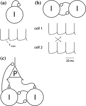
Fig. 2
The ING and PING mechanisms for neuronal synchronization in the gamma band (a) Consider one inhibitory neuron coupled to itself with a GABAergic synapse. If sufficiently depolarized, it will fire rhythmically with a frequency determined by the kinetics of the GABAergic feedback. b Consider two inhibitory neurons mutually coupled. When coupled they might fire either in phase or in anti-phase. It turns out that synchronized firing (in phase) typically is the most dynamically stable mode given realistic physiological parameters. This constitutes a mechanism for neuronal synchronization in the gamma band that generalizes to larger populations of interneurons. It is termed interneuronal network gamma (ING). c A second mechanism for the fast oscillations involves pyramidal neurons, and is termed pyramidal-interneuronal network gamma (PING). According to this mechanism the pyramidal neurons periodically excite the interneurons, which in return induce synchronized inhibitory post-synaptic potentials (IPSPs) in the pyramidal neurons
The PING mechanism (also referred to as the E-I, excitatory-inhibitory, model) constitutes another important principle by which neuronal oscillations can emerge in the gamma band. In contrast to the ING mechanism, the PING mechanism employs two different populations of cells: one excitatory and one inhibitory, reciprocally connected to each other (Whittington et al. 2000; Wilson and Cowan 1972; Ermentrout and Kopell 1998; Borgers and Kopell 2003). In the PING mechanism, AMPAergic projections of the excitatory population onto the inhibitory population provide fast excitation of the latter cells. These inhibitory cells, in turn, provide fast inhibition of the excitatory cells through GABAergic synapses. When the inhibition on the excitatory cells wears off, the excitatory cells fire. The excitatory firing results, a short delay later, in inhibitory firing, thus bringing the network into an oscillatory state. For this oscillatory state to happen, the strength of inhibition and excitation needs to be properly balanced. Note that the short delay between excitatory and inhibitory firing is the crucial factor for determining the oscillatory properties in this network (Borgers and Kopell 2003). This delay is composed of both axonal conduction and synaptic delays (Leung 1982).
For both ING and PING models, GABAergic interneurons are key players, a finding which is corroborated by the observation that GABA concentration in the brain predicts an individual’s peak gamma frequency (Muthukumaraswamy et al. 2009). Even though either of these two mechanisms could in principle explain all gamma oscillation phenomena in the brain, there is ample evidence that both of them are at work. For instance, when synaptic inhibition onto inhibitory cells is disabled in the mouse hippocampus, gamma activity is not significantly affected, providing evidence that some mechanism other than ING is at work (Wulff et al. 2009). In contrast, it is known that gamma oscillations are also prominent in structures that do not have dense excitatory-to-inhibitory connections (Brown et al. 2002; Fujisawa and Buzsaki 2011), indicating that PING cannot be the whole story. Thus, whether the PING or the ING mechanism is dominating might depend on the brain region and species (Tiesinga and Sejnowski 2009; Buzsaki and Wang 2012).
Given the likelihood that inhibitory interneurons are crucial for generating gamma oscillations, is anything known about the specific type of inhibition involved in this mechanism? Inhibitory interneurons can be broadly classified along two dimensions: fast-spiking versus non-fast-spiking, and soma-targeting versus dendrite-targeting. Several strands of evidence indicate that fast-spiking, soma-targeting basket cell interneurons (specifically, those that express parvalbumin (Kawaguchi et al. 1987)) are crucial in the generation of gamma rhythms (Bartos et al. 2007). These cells are abundant (Freund and Buzsaki 1996), form extensive interconnections amongst one another (Gulyas et al. 1999), and a single basket cell can project onto more than one thousand pyramidal cells (Cobb et al. 1995). These conditions enable basket cells to impose their gamma rhythm onto a pyramidal cell network; the population activity of the pyramidal cells then is reflected in the local field potential (LFP) and MEG signal. Furthermore, gamma activity is associated with strong perisomatic current sinks, consistent with the soma-targeting properties of basket cells (Mann et al. 2005). Finally, fast-spiking basket cells have resonance properties in the gamma range (Pike et al. 2000; Cardin et al. 2009) and typically produce ~1 spike per gamma cycle, phase-locked to the population rhythm (Gloveli et al. 2005). Further evidence shows that gamma-generating interneurons are likely coupled through shunting inhibitory synapses and by gap junctions, which increases their robustness against heterogeneous input (Vida et al. 2006; Bartos et al. 2007).
Apart from gamma oscillations, another high-frequency component of LFP and MEG signals can be distinguished. Sometimes referred to as high gamma, relatively broadband high-frequency activity (>85 Hz) is also known as epsilon activity (Freeman 2007; Belluscio et al. 2012) or the chi band (Miller et al. 2008). It is currently unclear to what extent this activity should be considered a rhythm. The high-frequency broadband spectral components might reflect the spectral fingerprint of neuronal spiking (Manning et al. 2009; Belluscio et al. 2012).
2.2 Beta Oscillations
Typically, beta oscillations (14–30 Hz) are considered to be generated by similar mechanisms as the gamma rhythm. A large-scale simulation of a network generating beta oscillations has been implemented (Traub et al. 1999), based on in vitro observations of hippocampal slices that alternate between gamma and beta states. It has been shown that the essential features of this large-scale network can be reproduced in a much simpler network, which bears strong resemblance to the PING mechanism of gamma generation (Kopell et al. 2000).
Imagine again the PING network described earlier, in which alternating balanced inhibitory and excitatory bursts between two coupled populations result in a network oscillating at gamma frequency. It turns out that only two changes need to be made to this model for it to generate beta oscillations: first, a slow potassium after-hyperpolarization (AHP) conductance is added to the excitatory cells, and, second, the excitatory cells have recurrent connections to themselves. When an excitatory cell has fired in this regime, it cannot fire again in the next gamma cycle, because then the AHP conductance prevents the cell’s membrane potential from reaching threshold. Only on the next cycle can the cell fire again. This phenomenon is known as “beat-skipping” and results in the excitatory cells synchronizing at a beta frequency that is half the frequency of the interneuronal gamma rhythm. Note that because the inhibitory cells receive phasic excitatory input from the pyramidal cells, when one pyramidal cell fires, other pyramidal cells on the next gamma cycle will be silenced by the recurrent inhibitory connection. This leads to a regime where, although each individual pyramidal cell fires in a beta rhythm, the population activity is still of gamma frequency. The additional change to the model, the addition of recurrent connections between excitatory cells, ensures the synchronization: because the excitatory cells excite one another, they will fire before the inhibition from the GABAergic cells arrives. The latter route requires two synapses, while the recurrent connection is monosynaptic. Thus, a “PINB” (pyramidal-interneuronal network beta) mechanism might explain the occurrence of beta oscillations in local neuronal networks (Kopell et al. 2000), such as in the hippocampus.
Just as PING is not the whole story for gamma, so PINB is not the whole story for beta. Beta oscillation amplitude over human sensorimotor cortex is increased when benzodiazepines are administered, while the oscillation frequency is decreased (Jensen et al. 2005). Benzodiazepines mainly act by increasing GABAergic conductances. In a PINB-regime, increasing GABAergic conductances has the effect of decreasing the spiking frequency of the inhibitory cells, thus allowing more of the excitatory cells to fire, which in turn then excites the inhibitory cells more, leading to an equilibrium in which the net effect on network frequency is negligible. Therefore, the PINB mechanism cannot explain the robustly observed effect of benzodiazepines on beta oscillations. In contrast, an “INB” mechanism, analogous to ING for gamma, is able to explain these findings: in this mechanism, excitation of the inhibitory cells is tonic, so the period of the inhibitory cells’ firing is determined only by the recurrent inhibitory connections. Since these become stronger under administration of benzodiazepines, the period of the inhibition becomes longer, in line with the observed results. As the period increases, a larger fraction of pyramidal cells will be released from inhibition during the refractory period. This explains the increase in beta power and decrease in frequency with benzodiazepines in sensorimotor areas observed in humans (Jensen et al. 2005).
2.3 Theta Oscillations
The mechanisms described above for the generation of gamma and beta oscillations are primarily local models: they describe how oscillations of a particular frequency can arise through interaction of neuronal populations within the same brain structure. This allows for related models to account for gamma and beta activity in different structures such as the hippocampus, entorhinal cortex, or neocortex. The lower-frequency theta oscillations (4-8 Hz), primarily (though not exclusively) observed in hippocampus, are typically thought to be generated by an interaction between several brain regions, and might not sufficiently be explained by a local model (Wang 2010).
Classically, the medial septum-diagonal band of Broca (MS-DBB) has been regarded as the crucial brain structure for the generation of the hippocampal theta rhythm, a notion which is corroborated by the observation that lesioning or inactivating the MS-DBB effectively obliterates theta in the rat brain (Stewart and Fox 1990). The MS-DBB provides a tonic cholinergic drive to the hippocampus which greatly influences the amplitude of the hippocampal theta rhythm (Lee et al. 1994). In addition, GABAergic interneurons in the MS-DBB project selectively onto hippocampal interneurons and these projections likely provide the phasic entrainment (Freund and Antal 1988; Buzsaki 2002). Although originally the MS-DBB was regarded as the pace-making structure for theta oscillations (i.e., it was thought that the MS-DBB generates theta by itself and then imposes its theta rhythm onto the regions to which it projects), later studies have found that interactions between the MS-DBB and the hippocampus, as well as intra-hippocampal processes, are just as essential for theta generation. For instance, it turns out that an in vitro preparation of an entire isolated hippocampus is still capable of generating theta oscillations (Goutagny et al. 2009). Furthermore, dendritic inhibition of pyramidal cells by oriens lacunosum-moleculare (OLM) interneurons, the presence of slow GABAA-receptors on hippocampal cells, and the value of several specific active membrane conductances all are important for the occurrence of hippocampal theta oscillations (Buzsaki 2002; Rotstein et al. 2005: Kopell et al. 2010; Wang 2010).
2.4 Alpha oscillations
Alpha oscillations (8-12 Hz) can be robustly observed in both the thalamus and the neocortex. Which of these two regions is the primary pacemaker of the alpha rhythm is still under debate. Generators of the alpha activity have been found with certainty in both thalamus and in neocortex (Lopes da Silva et al. 1980; Bollimunta et al. 2008, 2011). The neocortical alpha activity measured by MEG likely stems from an interaction between the thalamic and neocortical generators.
Most is known about the generation of thalamocortical (TC) alpha oscillations. The lateral geniculate nucleus (LGN) of the thalamus contains a particular set of TC neurons, the high-threshold bursting TC neurons, or HTC neurons. These neurons, coupled through gap junctions, fire bursts of spikes in synchrony with alpha oscillations in the field potential (Hughes and Crunelli 2005). However, this cannot be the whole story of TC alpha, since the main projections conveying visual information from thalamus to cortex are from relay-mode cells (Llinas and Jahnsen 1982), and not HTC cells. So how do the HTC and relay-mode cells interact? Extensive physiological and computational work has converged on the following model (Lorincz et al. 2009; Vijayan and Kopell 2012). HTC cells rhythmically excite thalamically local GABAergic interneurons, probably through axon collaterals. This causes these interneurons to also fire at alpha frequency. Depending on the strength of tonic excitation, the interneurons can fire in one of two modes: a rhythm of single spikes near the trough of an alpha cycle, or a rhythm of spike bursts near the peak of alpha. The interneurons project extensively to the relay-mode cells, thus resulting in an alpha-frequency occurrence of IPSPs on their membrane potential. Because of the two modes of firing of the interneurons, the relay-mode cells can send their information to the cortex in two distinct temporal framing regimes, i.e. at different alpha phases (Lorincz et al. 2009; Vijayan and Kopell 2012).
Apart from alpha activity, sleep spindles are also reflected in the frequency range of 10-15 Hz. These are thought to be generated by mechanisms related to the thalamocortical alpha oscillation, with some important differences: cells of the reticular nucleus are believed to be crucial for the spindle rhythm, and spindle activity emerges only in a regime of widespread (as opposed to sparse) inhibition, as would be expected for a sleep rhythm (Destexhe et al. 1993; Terman et al. 1996).
2.5 Delta Oscillations
Delta oscillations (1–4 Hz) are prominent during sleep, just like the spindle rhythm. A model has been proposed in which these two rhythms are generated by the same neuronal circuitry: an interaction between thalamic reticular (RE) cells, thalamocortical (TC) cells, and neocortical excitation of the reticular cells. In the generation of spindles, RE cells inhibit TC cells through GABAA and GABAB receptors. The TC cells project with excitatory connections to the cortex and the RE cells, and the cortex excites the RE cells. A network in this configuration generates spindle activity. When the conductance of the RE cells is changed such that they become less sensitive to the excitatory input of the TC cells, this causes the fast inhibition of the TC cells through GABAA-receptors to be functionally removed. The slow inhibition through GABAB is unaltered. This gives rise to a rhythm in the delta frequency range during sleep (Terman et al. 1996). Delta activity also occurs during wakefulness (e.g. Lakatos et al. 2008); however, few if any models have been developed for the generation of delta during wakefulness.
2.6 Cross-Frequency Interactions
In addition to observing oscillations in distinct frequency bands, one can also observe interactions between those oscillations. In Sect. 3.4, the different types of cross-frequency interactions that can be observed are outlined. The neuronal mechanisms underlying cross-frequency interactions are currently not well understood. One possibility for the observed coupling between the hippocampal theta rhythm and the neocortical gamma rhythm (Sirota et al. 2008) is that the hippocampal theta rhythm is imposed onto fast-spiking interneurons in the neocortex by direct anatomical projections (Tierney et al. 2004; Gabbott et al. 2002). These interneurons are crucial for the generation of the gamma rhythm, as explained in the section on gamma activity above. The number of interneuron network spikes per gamma cycle is proportional to the measured gamma amplitude in the local field potential (and thus the MEG signal). Since the interneuron network spike rate is determined by the input to the network, whenever this input is time-varying at a certain low frequency (e.g., theta), the gamma amplitude will be modulated at the same frequency (Spaak et al. 2012b; Wulff et al. 2009).
3 Methods for Characterizing Oscillations
An oscillation as measured by MEG can most simply be thought of as a stationary sinusoidal signal, varying across time at a particular frequency. However, such pure signals do not exist in the brain, but rather neural data are mixes of sinusoidal oscillations at varying frequencies whose peak amplitudes vary over time. This section describes how to compute meaningful quantities from these signals that characterize their frequency dependence and dynamics. Although the oscillations are recorded in the time domain (i.e., a signal that varies over time), often they can be better defined in the frequency domain (i.e., a signal whose amplitude and phase vary over frequency). The power spectral density (PSD) of a time series describes how its power (amplitude squared) is distributed with frequency. In this section, first we will describe the transformation of the raw (recorded) time series to the PSD and how the PSD is optimally computed for neuroscience applications. Second, we will describe how oscillations can alternatively be treated in the time domain and lastly, methods for computing within- and cross-frequency interactions. For further references on methods and computation, please see (Muthuswamy and Thakor 1998; Mitra and Pesaran 1999; Gross et al. 2013).
3.1 Power Spectral Density of Oscillatory Activity
Any time series can be re-written as a sum of sine waves with each wave having a frequency at the appropriate amplitude and phase. Vice versa, by knowing the amplitudes and phases of the waves, the original time series can be reconstructed. The amplitude and phase of the sine waves for all relevant frequencies can be determined from the Fourier Transform. Power is defined as the magnitude of the signal squared per time; thus the power spectral density describes how the squared amplitude for a given time window is distributed with frequency.
For discrete, digitized signals, such as those obtained from MEG, EEG, and invasive electrophysiological systems, the discrete Fourier Transform (DFT) is used to compute the amplitude and phase estimates for a finite number of frequencies. Thus, the PSD is the square of the DFT of a given discretized signal. The DFT is typically computed by the Fast Fourier Transform (FFT), a computationally fast and practical algorithm. Limits on the maximum frequency and the spacing of the estimated frequencies exist. First, the maximum frequency possible to be quantified, also called the Nyquist frequency, is half of the temporal sampling rate. For example, using a 1000 Hz sampling rate means that the maximum frequency at which information is estimable is at 500 Hz. If the underlying time signal contains information at a frequency higher than the Nyquist frequency, this information will bleed in at lower frequencies (termed “aliasing”), thus making this information irrecoverable and will corrupt the estimates at lower frequencies. Thus, it is imperative to low-pass filter the analog continuous signals prior to discretizing (Smith 1997). Indeed most commercial data acquisition systems will apply anti-aliasing filters via a lowpass filter at typically 1/4–1/3 of the sampling frequency. The second limit when converting recorded data to the frequency domain is the spacing between discrete frequencies. This spacing is referred to as the Rayleigh frequency and is equal to the inverse of the length of the temporal sampling window. For any finite signal, estimates of oscillatory power can only be obtained at integer multiples of the Rayleigh frequency (for example, for a 400 ms data segment, estimates will be obtained at 2.5, 5, 7.5 Hz, etc.) (Mitra and Pesaran 1999; Pesaran 2008).
In theory, the estimate of the power spectrum from the FFT of a finite data segment is biased, as the true spectrum can only be obtained from an infinitely long segment. In practice, however, directly applying the FFT to longer segments of data is less desirable for at least three reasons. It will require long computational time, it assumes stationarity of the underlying signal, and also it does not exhibit the expected property of a decrease in variance with increased data length. For a long segment, the noise will be represented at a high spectral resolution determined by the Rayleigh frequency, but not be averaged over nearby frequency bins. As such, while the frequency resolution increases with long data length, the noise variance of the spectral estimate is not improved. Welch’s method is one way to circumvent these concerns, by first “windowing” (i.e. cutting the data into N shorter equal-length segments) and then computing the power spectra per segment followed by averaging the spectra (Welch 1967). Figure 3 illustrates this, first by showing a long (20 s) time segment of a 20 Hz oscillation with added pink noise (Fig. 3a); a 1 s subset is shown in Fig. 3b. (Pink noise is noise drawn from a signal with a power spectral density following 1/f, in other words inversely proportional to frequency). If the FFT of the 20 s data is calculated (Fig. 3c), the peak at 20 Hz is strong, but also the noise is strong. In contrast, if the Welch method is used, whereby the FFTs of 20 (N = 20) segments, each 1 s long, are computed and averaged, the result is a smoothing over N adjacent frequency bins. This smoothing reduces the main peak at 20 Hz, but also reduces the noise, by the expected ratio of 1/√N. Effectively, one compromises frequency resolution when averaging over N bins, but typically the increased signal-to-noise ratio is preferred over a small Rayleigh frequency, since neural oscillations typically fluctuate in frequency. (Note that in Fig. 3, the short 1 s segments were padded to a length of 20 s prior to FFT; padding is discussed further down).
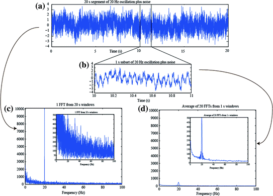
Fig. 3
Illustration of the averaging/smoothing over frequency provided by the Welch method using averaged spectra from shorter time windows. a A simulated 20 s long signal created from the addition of a 20 Hz sinusoid plus pink noise. b A zoomed in view of 1 s of the simulated signal. c The FFT of the data in (a). The inset is the same figure with a different y-scale. d The average of the 20 FFTs obtained from dividing the signal in (a) into 20 separate 1 s duration segments, with padding to 20 s length. The inset is the same figure with a different y-scale, but same y-scale as the inset in (c)
Segmenting has the further advantage of only assuming/requiring short-time stationarity within one segment, as variation over segments can be examined for non-stationarity. However, care should be taken that the segments do not become too short, as the practical minimal data segment length to sufficiently capture an oscillation is suggested to be about 3–5 times the length of the period of the frequency of interest. Thus, for example, a segment not much shorter than 400 ms should be used to estimate the power and/or phase at 10 Hz. Longer time segments may be advised if characterization of precise frequency estimates are desired (e.g., determining the peak frequency of the alpha oscillation during an eyes-closed resting condition to within 0.5 Hz precision would require a 2 s window). However, at least two concerns become apparent with the use of shorter time windows. The first is the increased Rayleigh frequency. In the example above, sacrificing a Rayleigh frequency of 0.05 Hz from a 20 s window to 1 Hz from a 1 s window is usually acceptable for most research questions; however, a Rayleigh frequency of 5 Hz, resulting from a window length of 200 ms, may not be sufficiently precise. To mitigate this, one may “pad” a time window with extra zeros resulting in a desired Rayleigh frequency. New information has not been gained at these intermediary frequency bins; the improved frequency resolution is a consequence of spectral interpolation. However, padding allows a spectrally smoothed representation to be depicted. In the situation of unequal time segments, for example due to unequal trial lengths between stimulus and response time, padding each segment to an equal length is necessary if these trials are to be averaged in the frequency domain and thus at the same frequency bins. The effect of padding is illustrated in Fig. 4
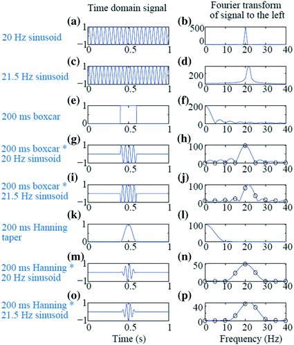
Fig. 4
Effect of window length, zero padding, and tapering on short window Fourier Transform. a 20 Hz sinusoid over 1 s. b FFT of (a). c 21.5 Hz sinusoid over 1 s. d FFT of (c); note the spectral leakage. e Boxcar window of length 200 ms. f FFT of (e). g Sinusoid from (a) multiplied by boxcar from (e). h Blue line is the FFT of 1 s padded segment from (g); black circles are the FFT from the 200 ms segment without padding. i Sinusoid from (c) multiplied by boxcar from (e). j Blue line is the FFT of 1 s padded segment from (i); black circles are the FFT from the 200 ms segment without padding. Again notice the bleeding. k Hanning taper of length 200 ms. l FFT of (k). m 20 Hz sinusoid from A multiplied by Hanning taper of (k). n FFT of (m), with the blue line resulting from padding to 1 s and the black circles from no padding of the 200 ms segment. o 21.5 Hz sinusoid from (c) multiplied by the Hanning taper of (k). p FFT of (o), with the blue line resulting from padding to 1 s and the black circles from no padding of the 200 ms segment. The Hanning taper effectively resolved the leakage but with the trade-off of increased spectral smoothing
A second problem with shorter time windows is that more blurring (spectral leakage) of the PSD can occur. The original Fourier Transform assumes an infinitely long signal with periodic components. However, when a segmented time window is used, this is implicitly the multiplication of a boxcar-shaped window (zeroes everywhere except a segment of ones) with the original signal. Since multiplication in the time domain is equivalent to convolution in the frequency domain, the FFT of a windowed time series appears as the convolution of the FFT of the original signal (for example, a stick, or delta function, at 20 Hz for a pure 20 Hz sinusoid) with the FFT of a boxcar, which is a sinc function. The resulting power spectral density contains power in the “tails” of the sinc function, outside the main peak of 20 Hz. This is illustrated in the example in Fig. 4. The time domain (left column) and frequency domain (right column) of several signals are shown. Figure 4a and 4c show sinusoids at 20 Hz and 21.5 Hz, respectively, with a sampling rate of 1000 Hz for duration of 1 s. The Rayleigh frequency is thus 1 Hz and the 20 Hz sinusoid can be well captured in the PSD as a sharp peak at 20 Hz and no power elsewhere (Fig. 4b). However, since the 21.5 Hz sinusoid contains its power at a frequency not at a multiple of the Rayleigh frequency, then the corresponding PSD exhibits a blurred peak near the true frequency but also power in other bands quite some distance from the true peak (Fig. 4d). The situation is worsened by using a shorter time window of 200 ms (sufficiently long to capture at least three periods of oscillation for both 20 Hz and 21.5 Hz), as shown in Fig 4g, i. The Rayleigh frequency is now 5 Hz; the PSD at every 5 Hz is shown in Figs 4h, j indicated by the black circles. The blue lines in these subfigures are computed from “zero padding” the 200 ms signal to a full 1 s length (as depicted in Fig. 4g, i). In Fig. 4h, the PSD of the 20 Hz sinusoid is again well captured with the peak power at 20 Hz and no power at the other sampled frequencies for the time window 200 ms; however, the FFT of the padded signal shows the leakage effects of the boxcar window. Furthermore, in Fig. 4j the bleeding of power to frequencies away from the true 21.5 Hz is strong, both in the unpadded (black circles) and padded (blue line) results.
An operation known as tapering can be used to mitigate the effect of the bleeding into far-away frequencies due to shorter time windows. Tapering is the explicit multiplication of the signal with some taper or window function, rather than relying on the implicit multiplication with a boxcar. Smoothing the sharp rise/fall of the boxcar edge leads to reduced leakage into further away frequencies. Tapering results in local smoothing of the peak frequency and thus assumes similarity of power in nearby frequencies (an assumption which is usually justified when analyzing brain signals). A common function used is the Hanning taper. A 200 ms version of the Hanning taper with zeros padded on either side is shown in Fig. 4k and its FFT is shown in Fig. 4l. When multiplying the windowed sinusoids by the Hanning taper (Fig. 4m, o), the resulting FFT of the sinusoids (Fig. 4n, p) now appear as the stick (delta function) at 20 or 21.5 Hz convolved with the smooth curve of Fig. 4l, rather than convolved with the bumpy curve of the sinc function in Fig. 4f. The short window of 200 ms still limits the Rayleigh frequency to 5 Hz and there is still some bleeding at nearby frequencies (e.g. at 15 and 25 Hz); however, the leakage at 10–30 Hz is greatly reduced. It is often recommended to demean before FFT as the baseline (DC) component can leak to other frequency bands.
The choice of which taper to use is based on the assumptions of the underlying true PSD. The Hanning taper illustrated minimizes the spectral leakage in the tails (also referred to as leakage in the side lobes) but results in a fairly wide blur around the true spectral peak (also referred to as a wide main lobe). Ideally, the taper choice should match the expected underlying spectral width. For example, in the alpha band of 8–12 Hz with a 4 Hz bandwidth, the Hanning taper over a 400 ms window gives a suitable match of the width of the main lobe (in fact, one roughly twice as narrow as that depicted in Fig. 4l, since the longer that the Hanning taper is in time, the narrower the lobe is in frequency). Other functions such as the Hamming taper can also be used. The Hanning, Hamming and other tapers differ from each other in their characteristics of relative suppression of the leakage in near and far frequency bands and width of the main lobe. Please see Smith (1997) for a detailed discussion.
When considering neural responses in the gamma band, they are often broadband, for example from 60–80 Hz. In this case, one commonly uses a set of tapers, known as the Slepian or discrete prolate spheroidal sequences (DPSS) or simply “multitapers” (Slepian and Pollak 1961), which are a set of mutually orthogonal vectors with optimal desired spectral properties. The number of tapers used is determined by the length of the time window (Δt) and the desired frequency bandwidth (Δf), with the formula: K = 2*Δt*Δf – 1, where K is the number of tapers (Percival and Walden 1993). Ideally at least three tapers should be used. A set of four DPSS are shown in Fig. 5. The result of using the multitaper method is a wider but specific passband with minimal leakage in the stopbands. In other words, the spectral properties are ideal for a broadband but yet band-limited response in the gamma band. The choice of data segment length and desired bandwidth of the multitapers is important, but to advise specific settings that are generally applicable is not possible. Rather, iteration and initial exploration of the data is recommended, for example, to determine whether a wide-band response is actually two distinct bands near each other. Further discussion of Fourier analysis for neural signals can be found in Pesaran (2008).
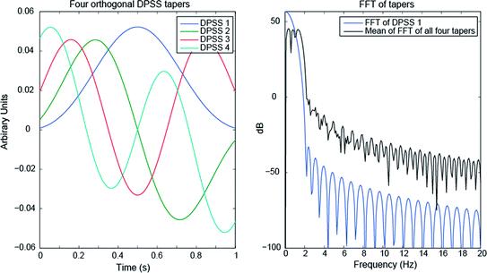
Fig. 5
Orthogonal DPSS tapers over a 1 s window (left) and their spectral density (right), with zero padding to 10 s length. The black line in the right figure is the average of the FFT of each taper, which indicates the effective result of using all four together
3.2 Time Domain Characterization of Oscillations
Rather than computing the FFT of a time-windowed signal to obtain its PSD across all frequencies, another option is to band-pass filter the data so as to obtain a time domain signal containing only frequencies of some band of interest. The success of this method depends on the characteristics of the filter which, similar to the discussion of tapers above, depend on passing the desired frequencies (in the “pass-band”) with as close to unity gain as possible and suppressing the non-desired frequencies (in the “stop-band”) with as close to full attenuation as possible (see Fig. 6). The “transition-band” refers to the frequencies in between the pass-band and stop-band for which the gain is neither zero nor unity. Four filter types are named according to the relative position(s) of their pass-band and stop-band: low-pass (Fig. 6), high-pass, band-pass and band-reject. In reality, filters are not perfect, and thus three important characteristics of filters are roll-off between the pass-band and reject-band, amount of ripple in the pass-band, and amount of attenuation in the stop-band. For more information on digital filtering, please see Smith (1997).
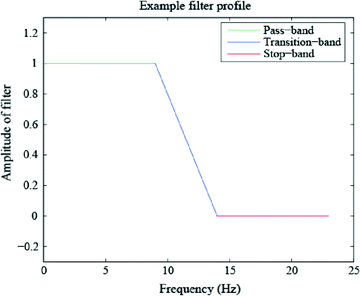
Fig. 6
Portions of a low-pass filter which correspond to the pass-band (unity amplification), transition-band (neither unity amplification nor full suppression), and the stop-band (full suppression). Similarly, a high-pass, band-pass and band-stop filter can be constructed
While the characterization above (low-pass, high-pass etc.) applies to the desired behavior of the filter, another characterization of filters is the type of implementation used: “infinite impulse response” (IIR) or “finite impulse response” (FIR). We do not intend to provide a mathematical explanation of these types and how they differ, but rather to introduce and discuss trade-offs of commonly used filters in neuroscience. For further details please see (Smith 1997). The Butterworth filter is a commonly used IIR filter. Some considerations as to whether to use an IIR or FIR filter are that IIR filters tend to have a flat frequency response but a shallow drop-off in the frequency domain and indirect control over time and frequency resolution, whereas FIR filters tend to have precise control over time and frequency resolution and a sharp drop-off in the frequency domain, but have an “oscillating” response in the frequency stop-band. The order of the filter is important as well, as it relates to the amount of temporal lag of the convolution kernel as well as computation time. One important criterion is to use a filter that will preserve the phase of the signal (a “zero-phase filter”) since the phase of the oscillation can be of important functional importance. A zero-phase filter is often implemented by applying two linear-phase filters in succession, where the second “un-does” the phase shift of the first. However, it is important to know that no filter is perfect and thus by applying the same filter twice to obtain zero-phase, the amplitude is reduced twice as strongly in the pass-band. Thus when comparing amplitudes across conditions, it is imperative to use the same filtering and other preprocessing.
Related posts:

Stay updated, free articles. Join our Telegram channel

Full access? Get Clinical Tree


