Bhawna Satija, Rama Anand, Smita Manchanda, Sudeshna Malakar The word tomography is derived from ancient Greek word Tomos meaning “slice, section” and graphein which means “to write” or, in this context as well, “to describe.” So, in simpler terms tomography means imaging of an object by analyzing its slices. Utilization of computers for this process confers the modern terminology of Computed Tomography (CT). History: The first commercial CT scanner was invented by Sir Godfrey Newbold Hounsfield in Hayes, United Kingdom, at EMI Central Research Laboratories. Hounsfield formulated this idea in 1967 and the first patient brain-scan was done in 1971. In 1979, he shared the Nobel Prize in Physiology & Medicine with Allan MacLeod Cormack, Physics Professor at Tufts University in Massachusetts, who developed mathematical solutions to CT-related problems. Table 1.9.1 gives a brief chronology of events in the development of the modern day CT scanners. Computed tomography (CT) scan machines use ionizing radiation in the form of X-rays, a powerful form of electromagnetic energy. The combination of X-ray radiation and radiation detectors integrated with a computer generates cross-sectional image of any part of the body. Important tissue details can be masked by overlapping tissues in the human body in planar projected images of the patient. CT can yield sequential images in thin consecutive slices of the patient and provide three-dimensional localization. Computed tomography utilizes multiple projections of an object to reconstruct its internal structure. The image in CT is derived by measuring the attenuation of X-rays traversing the patient in different directions and mathematically calculating the linear attenuation coefficients, µ, over the slice dimension. A thin cross section of human body is scanned with a narrow beam of X-rays and transmitted radiation is measured to obtain ray projections. The image receptor comprises of an array of multiple small separate receptors. The readings from these receptors which actually represent the linear attenuation coefficients of X-ray photons are processed by a computer to reconstruct a tomogram of the patient. Since its inception, there has been a change in the arrangement of the X-ray tube and the detectors over years, with the primary objective of reducing scan time. In addition to improved temporal resolution, the technical advancement has been from a slice based to a volume-based technique. The different technical solutions are termed “generations” and these generations primarily describe the X-ray and detector configuration. First-generation CT had a translate rotate type of movement between the X-ray tube detector combination. It consisted of only single detector per slice and the X-ray tube had a pencil beam geometry (Fig. 1.9.1). This was primarily designed for scanning the brain. The detector material was made of sodium iodide scintillation crystals coupled with photomultiplier tube. The patient in this type of scanner was stationary whereas the gantry moved in rotatory movements. Gantry used to translate a total of 180 degrees with 01-degree rotation between each translate. The time taken for a single scan was approximately 4.5 min, thus regions where patient motion is minimum (e.g. head) could only be imaged. This was another rotate translate type of scanner. This had a faster scanning time as compared to first generation. It had a narrow fan beam type of geometry (3 degree–10 degree) with multiple detectors (up to 30) (Fig. 1.9.2). The rotatory steps taken by this type of scanner were larger (around 30 degrees as compared to 1 degree in first generation). Scan time for acquiring one scan was reduced to one third. It has a rotate rotate type of tube detector combination. Both the tube and detector rotate in a fan beam geometry. The number of detectors is much more as compared to second generation (up to 700 in number) and arranged in a curvilinear array (Fig. 1.9.3). The detector material is made of xenon or scintillation crystals. This scanner is much faster and can produce an image in few seconds with recent versions capable of less than a second scan time. One important disadvantage of third-generation CT scanners is production of ring artefact. It occurs due to miscalibration or failure of one or more detector elements and can be removed by software corrected image reconstruction algorithms. It has a rotate fixed type of geometry where the detectors are fixed in the form of a ring around the patient and the X-ray tubes rotate inside the detector ring. The X-ray tube has a fan beam type of geometry with more than 2000 detectors (Fig. 1.9.4). As the alignment of detectors with X-ray tube is continuously changing, it avoids the ring artefact seen due to detector misalignment in third-generation scanners. These scanners are capable of sub-second imaging time. Table 1.9.2 summarizes important differences between various generations of CT scanners. It is ultrafast type of scanner with fixed fixed type of geometry (Fig. 1.9.5). Here magnetic focussing of the electron beam is done. The scanning time is as low as 20msec/slice. This scanner has superior temporal resolution and is used for cardiac imaging. The development of helical/spiral CT revolutionized CT imaging by allowing acquisition of true three-dimensional images in a single breath-hold. Here, the X-ray tube circles the patient while the examination table moves continuously. The X-ray beam from the CT traces a helical path around the patient (Fig. 1.9.6), hence the name. The helical path acquires three-dimensional data, which can further be utilized to reconstruct sequential images for a stack. The modern CT protocols use helical acquisition due to its speed which results in reduced misregistration from patient movement and breathing. The major technological advancements that have led to the development of the fast-helical scanners are A slip ring is an electromechanical technology that enables the transmission of power and electrical signals from a stationary to a rotating structure. This transmission of power is made via electrical connections made by stationary brushes pressing against rotating circular conductors. This technology is also called “rotary electrical joint” and “electric swivel” technology. A slip ring can be used in any electromechanical system that requires unrestrained, intermittent or continuous rotation while transmitting power and/or data. CT Slip ring technology was introduced to enable helical (continuous rotating) scanning. Prior to the introduction of slip rings, only axial scanning was possible (which had the need to stop/reverse direction of rotation, after no more than 700 degrees rotation due to the finite length of the attached cables.) Slip ring technology eliminated the need for cables and enabled the continuous rotation of the gantry components, eliminating the inter-scan delay. The slip ring technology led to the reduction in inter-scan delay, thereby increasing thermal demands on the X-ray tubes. In order to meet these requirements, X-ray tubes with increased anode heat capacities (5–8 MHU), improved heat dissipation rates and reduced mass were designed. The larger heat capacity was achieved by using thick graphite backed target discs, larger anode diameters (200 mm or more), high speed rotors and metal housing with ceramic insulators. Helical CT involves continuous acquisition of projection data through continuous rotation of X-ray tube and detectors and simultaneous translation of patient through the gantry. These projections obtained from a helical motion do not lie in a single plane and thus conventional reconstruction algorithms cannot be employed. Will Kalender addressed this problem by developing methods to generate projections in a single plane and thus enabling utilization of conventional back projection. This method is called interpolation algorithm, which means estimating a value between known values. This method offered significant advantages. Once the volume data was acquired in single breath hold, the reconstruction plane could be placed in any desired position to obtain 3D reconstruction data free of misregistration artefacts. This led to acquisition of 3D volumes and true 3D radiography could be realized. This also rendered improved z-axis sampling without any additional radiation dose to the patient. The most important advantages of helical CT over conventional CT are New detector technologies were introduced and many terms were used to describe this new technology: multidetector-row CT, multirow helical CT, multidetector helical CT and multislice helical CT (Fig. 1.9.7). However, the term multislice and multidetector CT are the more commonly used terms used in clinical practice. The word multislice and multisection in MDCT implies that depending on the detector design comprising of multiple rows of detectors, more than one image slice or image section is acquired for each time the gantry completes a rotation. The basic difference between MDCT scanners and a single slice helical scanner is the consequence of the detector array design (Fig. 1.9.8). The replacement of a single detector row by four or more rows augments the data acquisition capability significantly. Conventionally, a single slice spiral CT scanner utilizes a single tube source that activates only one row of detectors irrespective of the X-ray beam collimation, measuring about 20 mm in length (along Z or long axis). In MDCT, this is substituted by multiple row of detectors called a detector array that allows simultaneous acquisition of multiple slices during one single gantry rotation. The different types of detector array matrices commercially available include fixed, adaptive and mixed types. A fixed detector array has uniform thickness matrix elements, whereas an adaptive matrix has elements wider away from the centre. A mixed array has all matrix of similar size with exception of few thinner ones at centre. The array design is a crucial entity in MDCT scanner as it defines minimum slice width, number of slices possible with minimum width, range of slices available and maximum length imaged in a particular direction. This detector array coupled with a slip ring allows continuous rotation and leads to significant reduction in rotation time of tube detector assembly from 1 to 0.5 s. Two essential features of MDCT technology Improved scan speed enables a much comprehensive coverage in a single breath hold with significant reduction in patient movement artefacts and thus also facilitates optimum use of contrast media. The other important characteristic of MDCT is “isotropic” imaging, which is defined as identical resolution of an imaged voxel in all dimensions. This valuable attribute plays a pivotal role in 3D imaging by eliminating the stair step artefacts of single slice CT and helical CT along with good definition of the anatomical edges. This represents the relationship between patient couch movement and X-ray beam width. It is the distance travelled by the table during one 360 degree gantry rotation divided by the collimated section thickness. In Single-row detector helical CT scanners Pitch is expressed as a ratio, such as 0.5:1, 1:1, 2:1, etc. The pitch factor relates the volume coverage speed to the thinnest sections that can be reconstructed. The radiation dose is inversely proportional to the pitch. Increasing the pitch above 1:1 increases the volume of tissue imaged at a given time but reduces image quality. In Multi-row detector helical CT scanners where N = Number of detector rows. The mechanism of image formation in CT depends on the receptors measuring the X-rays coming through a slice of the patient in different positions, forming one projection of the patient. The slice through which X-rays pass is divided into tiny blocks known as voxels or volume elements. The reading of any one receptor is a measure of the attenuation in different voxels along the path of a particular ray. Attenuation measurements are used to quantify the fraction of radiation removed in passing through a given amount of specific material of thickness Δx. In a homogeneous object with monochromatic radiation, the receptor reading, i.e. attenuation, is equal to I = Ioe−μ∆x where Since patient is an inhomogeneous object, each attenuation measurement is called a ray sum as it measures sum of the individual attenuation of all materials (voxels) along the path. The transmitted intensity is then given by I = I ° e − ∑ μ i Δx − ∑ μ i Δx = − ( μ 1 + μ 2 + μ 3 + …………. μ k ) Δ x Once the data from sets of projection profiles through all volume elements (voxels) in a slice of the patient for sufficient numbers of rotation angles (projections) is obtained, it is possible to calculate the average linear attenuation coefficient, µ, for each voxel. This procedure is called reconstruction. Each value of µ is assigned a grey scale value on the display-monitor and is presented in a square picture element (pixel) of the image. The computer reconstructs an image, a matrix of µ-values for all voxels in a slice perpendicular to the rotation axis. Thousands of equations are required to calculate the linear attenuation coefficients of all the pixels in the image matrix. In order to achieve this task at a fast speed without compromising the accuracy, various reconstruction algorithms are used. Filtered back projection (convolution method): Filtered back projection, one of the most widely used image reconstruction technique in present day CT scanners, utilizes a convolution filter to diminish the blurring associated with back projection. The frequencies responsible for blurring are removed with the help of filter before the data back projected. It is fast, however, limited by noise and artefact creation. 2D Fourier transformation: It is based on the Fourier slice theorem which utilizes frequency domain analysis of the problem. In the spatial domain, CT utilizes relationship between a 2D image and its set of one-dimensional views. The problem can be analyzed in frequency domain by obtaining a 2D Fourier transform of the image and one-dimensional Fourier transform of its views. The relationship of an image with its views is much simpler in frequency domain and forms the basis of Fourier transformation. The image in CT is derived from the stored electronic information obtained from attenuation of X-rays and is displayed as a matrix of intensities. The cross-sectional portion of the body which is scanned for to generate CT image is called a slice. The slice comprises of width and thus volume. The width of the X-ray beam determines the slice width. The image format comprises of many individual cells, each assigned a number and representing an optical density or brightness level on the monitor. Matrix is a two-dimensional array of numbers arranged in rows and columns. The original EMI scanner comprised of an 80 × 80 matrix, thereby providing 6400 individual cells of information. Currently available systems provide matrices of 512 × 512, 1024 × 1024, 2048 × 2048, thus providing large number of cells of information. Each individual element in the image matrix is representative of a three-dimensional volume element in the object, called a VOXEL or volume element. The depth of a voxel is equal to slice thickness. The VOXEL is portrayed in the CT image as a two-dimensional element called PIXEL (picture element). Thus, every pixel on the computer monitor is derived from a voxel inside the patient. Each pixel of the image matrix contains a number which represents the X-ray attenuation in the corresponding voxel of the object. This number represents the CT number which is actually a measure of the average linear attenuation coefficient (µ), between tube and detectors. Attenuation coefficient reflects the degree to which the X-ray intensity is reduced by a material that is being imaged. The linear attenuation coefficient (μ) of each voxel is determined by The computer calculates linear attenuation coefficient of each pixel and further converts it to new digital number which is known as CT number. The CT number is calculated by the equation CT number = K ( μ P − μ w ) μ w where From the above equation, CT number for water is always zero. The CT numbers are normalized to attenuation of water, which considerably reduces the difference with photon energy of X-rays, especially for materials with atomic numbers similar to that of water. When K is 1000, the CT numbers are termed Hounsfield Units (HU). HU value of various tissues can be measured by drawing ROI – region of interest. These measurements provide information about the tissue composition. Windowing and Grey Scale: The CT numbers are assigned different shades of grey on a grey scale to derive a visual image. Each shade of grey represents the X-ray attenuation within the corresponding voxel (Fig. 1.9.10). Modern CT equipment that are being used today have a capacity of around 4096 gray tones. The monitor that is used for viewing can display maximum of around 256 gray tones. However, the human eye is able to discriminate only ~20 Gray tones. High quality image generation is indispensable for obtaining maximum diagnostic information from the CT images used in medical imaging. The discernibility of diagnostically important structures in a CT image defines image quality. High quality images usually imply higher radiation dose to the patient. It is imperative to understand image quality assessment tools in CT to optimize low radiation dose in a way that it is consistent with image quality of adequate diagnostic efficacy. The factors that determine the quality of image in CT are intimately related to each other and include image noise, image resolution, presence of artefacts and patient exposure. When a homogeneous medium is imaged under ideal circumstances, each point on detector should receive same number of photons and each pixel should have a same value. However, this does not happen, therefore the CT numbers always have a range of values above or below the ideal value for that substance. This variation in CT numbers greater or less than the average value accounts for the noise of the system. Noise would be zero if all the pixel values were equal. Noise is seen as irregular granular pattern in the image, which may show alternating thin bright and dark streaks. Image noise refers to the graininess of the image. Statistically, noise is described as a standard deviation and symbolized by σ. Noise ( σ ) = ∑ ( x i − x ¯ ) n − 1 2 xi = each CT volume n = number of CT values averaged The precise way by which noise can be reduced in the system is to increase the number of absorbed photons by the detector which in turn implies increasing the X-ray dose to the patient. Most of the noise we see in our images is a result of statistical fluctuation and unrelated to the models used for mathematical reconstruction. The number of photons per pixel is in turn dependent on many factors: A shorter scan time is desirable to decrease patient motion. However, scan times can only be shortened to a certain extent as this reduces image precision. The reduction in pixel and voxel size decreases the image noise, however also leads to a significant increase in patient exposure. So, there is a need for obtaining an optimum balance between the acceptable pixel size and image noise. The noise is also less with a smaller matrix (i.e. 60 × 60) than a larger matrix (180 × 180). Another factor is the “Field size” which controls the maximum size of the anatomical part that can be examined at once by a particular scanner. Smaller field sizes can be used for high resolution images. Resolution has two components; spatial and contrast resolution. These two parameters are intrinsically related to one another which in turn is also related to the radiation dose absorbed by the detector (i.e. quantum mottle/noise). Improving spatial resolution beyond a certain level will increase noise in the system which then shall decrease contrast resolution. On the other hand, to improve contrast resolution by increasing scan times and also imparting larger doses may decrease spatial resolution by increasing the effects of patient motion. The derivation of Computed Tomography image involves physical measurements of the attenuation of X-ray beam traversing the patient followed by mathematical calculations of the linear attenuation coefficient (µ). These calculations are based on assumptions and may not correspond to actual information. This creates deviation of the measurement and reconstruction of the µ-values from true attenuation coefficients of the object resulting in artefacts. Artefacts in the image represent patterns which do not exist in patient’s true anatomy. The pattern of artefacts that are created can be described as streaking, shading, rings and distortion. The artefacts seen in CT image can be due to various factors. Patient Related
1.9: Computed tomography
Year
Development
1924
Johann Radon formulated the mathematical theory of tomographic image reconstruction.
1930
A. Vallebona constructed equipment and published 1st clinical body section imaging material.
1963
A. McLeod Cormack developed the theoretical underpinnings of CT scanning.
1971
1st generation CT: commercial CT introduced by Sir Godfrey Hounsfield.
1972
EMI scanner was introduced as clinical system of cranial examination.
1974
2nd generation CT.
1975
3rd generation CT.
1976
4th generation CT.
1979
Cormack & Hounsfield shared the noble prize in physiology or medicine.
1980
5th generation cardiac CT.
1989
Single-row CT.
1991
Spiral CT was introduced.
1994
Double row spiral CT.
1998
Multidetector CT.
2004
16 row spiral CT.
2006
Dual source CT introduced.
2007
320 row spiral CT.
Principles of computed tomography
Principles
Generations of CT
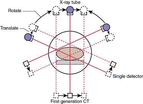
First-generation CT
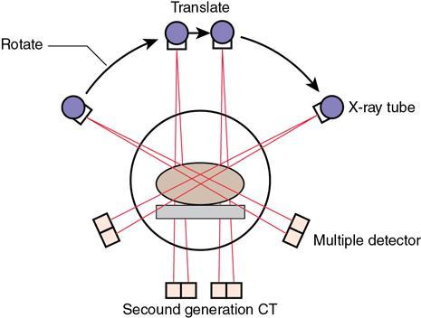
Second-generation CT
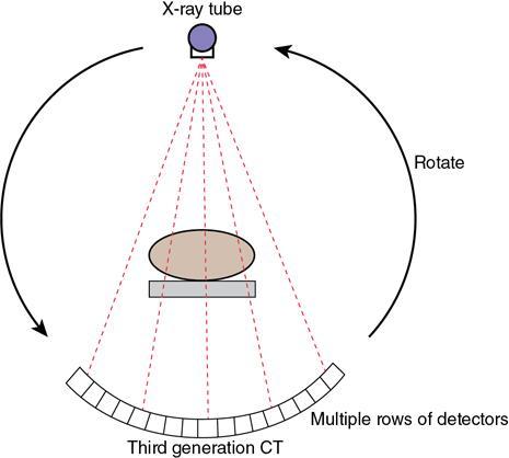
Third-generation CT
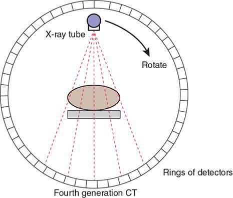
Fourth-generation CT
S. No.
Parameter
1st Generation
2nd Generation
3rd Generation
4th Generation
1
X-ray beam shape
Pencil beam
Narrow fan beam
Wide fan beam to cover FOV
Wide fan beam to cover FOV
2
Number of detectors
Single
Multiple (up to 30)
Multiple (200–700)
Multiple >2000
3
Tube detector movement
Rotate-translate
Rotate translate
Rotate-fixed
Rotate-rotate
4
Detector collimation
None
Collimated to source direction
Collimated to source direction
Collimation not possible
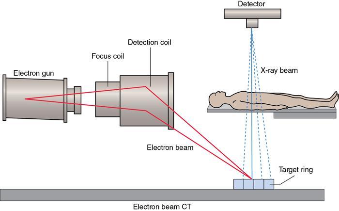
Fifth-generation CT (electron beam CT)
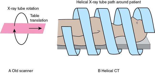
Helical CT/spiral CT
Slip ring technology
High power X-ray tubes
Data interpolation algorithms
Advantages of spiral CT
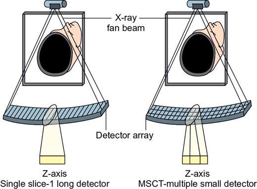
MDCT
Advantages of MDCT
Helical pitch
Image reconstruction


Reconstruction process
Reconstruction algorithms used in CT
Image analysis
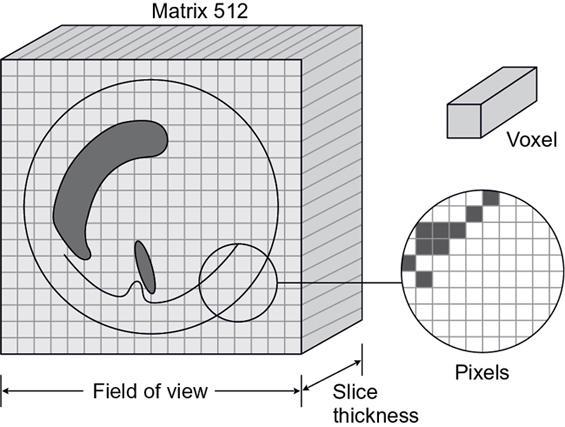
Matrix, pixel and voxel concept (Fig. 1.9.9)
CT numbers
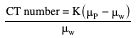
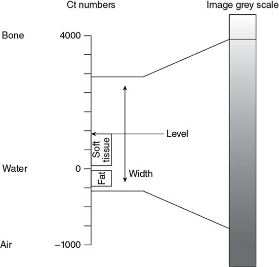
Image quality and radiation dose
Quantum mottle (noise)
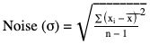
x ¯  = average of at least 100 values
Resolution
CT artefacts
Related posts:


Stay updated, free articles. Join our Telegram channel

Full access? Get Clinical Tree


