Tomographic Angiography
Mathias Prokop


ECG SYNCHRONIZATION AND CARDIAC COMPUTED TOMOGRAPHIC ANGIOGRAPHY


Computed tomographic angiography (CTA) is one of the big success stories in diagnostic radiology. CTA was developed shortly after the introduction of spiral (helical) CT scanning in the early 1990s. Spiral CT had made it possible to cover body regions so rapidly that the transient enhancement of the vascular system following intravenous contrast injection could be captured during one scan. With the introduction of multidetector-row technology, CTA gained a tremendous boost and quickly became an easy-to-perform standard technique for vascular imaging.
Over the years, CTA—together with magnetic resonance angiography—has taken over most diagnostic vascular procedures from invasive catheter angiography, first for the aorta and the pulmonary arteries; later for the carotids, renal, and splanchnic arteries; and recently also for peripheral arteries and the circle of Willis. Most recently, CTA of the coronaries has been developed. While coronary CTA is still technically challenging, it also holds the promise to substitute for part of diagnostic cardiac catheter angiographies.
CTA has the advantage that it can be highly standardized, which makes it a very fast and robust procedure that is the technique of choice in many acute vascular diseases. It provides three-dimensional information with a comparatively high spatial resolution and allows for simultaneous evaluation of the vascular lumen as well as the vessel wall and the surrounding structures. In fact, every arterial phase CT can potentially serve as an arterial CTA, while a portal phase scan can serve as a portal venous CTA.
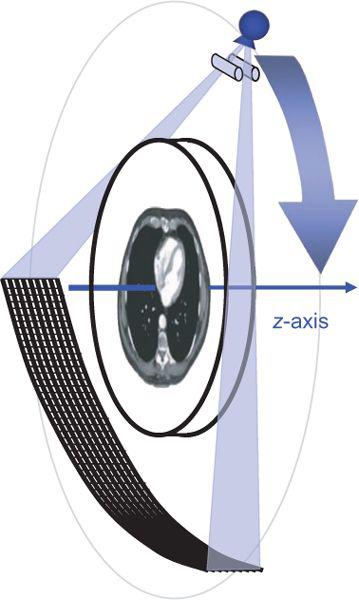
FIGURE 1-1 Principle of current CT scanners: A thin fan-shaped beam rotates around the body and is detected by a synchronously rotating detector array. (From M. Prokop et al. Spiral and Multislice CT of the Body. Thieme Medical Publishers 2003, with permission.)
CT technology has seen more rapid improvements than other radiological techniques: over the past decade, scanner performance doubled approximately every two years. While CT technology nowadays is more than sufficient for standard CTA applications, further developments focus on improvement of quality and robustness of coronary CTA as well as CT perfusion imaging.
This chapter will provide the basic understanding of CT technology as it relates to CTA as well as show how to optimize scanner parameter settings, discuss various trade-offs, and suggest solutions to typical problems and pitfalls encountered in clinical practice.
BASIC CONCEPTS OF COMPUTED TOMOGRAPHY
Computed tomography is an x-ray tomographic technique in which an x-ray source rotates around the body and an x-ray beam passes through the patient from various directions (Fig. 1-1). A mathematical image reconstruction (inverse Radon transformation) uses the x-ray attenuation along each of the many paths through the body (the CT raw data) to calculate the local attenuation at each point within the acquisition volume. The local attenuation coefficients are normalized to yield CT numbers for every point of the image matrix. These CT image data are finally converted into shades of gray that are displayed as an image.
The first two generations of CT scanner geometries were already abandoned in the late 1970s and were substituted by third- and fourth-generation scanners. With the advent of multidetector-row CT, only third-generation geometry is still available. In these scanners, an x-ray tube and a detector array rotate synchronously around the patient. Parallel collimation is used to shape the x-ray beam to a thin fan, which defines the total thickness of the acquired transaxial volume (Fig. 1-1).
Apart from the first scanner generations in the 1970s, which had two parallel detector arrays, later scanners used a single detector array for measuring the intensity of the attenuated radiation as it emerged from the body. In these single detector-row scanners, the thickness of the acquired section could be varied by changing the collimated width of the x-ray beam. For thinner section collimation, only part of the detector array was exposed (Fig. 1-2A). In the early 1990s, one vendor introduced a dual slice system, in which the detector array was split in half so that two sections were exposed simultaneously (Fig. 1-2B). In the late 1990s, multidetector-row scanners were developed that consisted of multiple parallel arrays that could be combined so that four simultaneous sections could be acquired (Fig. 1-2C). Development went on rapidly, and currently, 128-row scanners are on the market.
In the 1970s and 1980s, the scan volume was covered in a stepwise manner: After acquiring a transaxial section, the table was moved by a certain amount (usually the section thickness and the next of these sequential scans was performed (Fig. 1-3A). This scanning technique was slow and suffered from discontinuities at the border between sections whenever there was motion between consecutive scans.
With the advent of scanners with continuously rotating x-ray tubes, it became possible to acquire a data volume in continuous fashion: Raw data was captured during multiple rotations while the patient table moved through the scan plane (Fig. 1-3B). This technology, which was named spiral or helical CT, required suitable interpolation techniques to compensate for motion while allowing for reconstruction of a complete three-dimensional data set consisting of overlapping axial images. It became the basis of CT angiography because it avoided step artifacts due to suboptimum registration (for example, as a result of inconsistent depth of inspiration between consecutive sections and had the advantage that a larger volume could be imaged rapidly and continuously so that transient phases of contrast enhancement could be captured within one scan.
Dynamic scanning is the third scanning technique available in CT: Here, the table remains stationary, and the scanned sections are exposed repeatedly to image dynamic processes such as the enhancement after intravenous contrast injection (Fig. 1-3C). Dynamic scanning can be used to find the optimum starting point for a CTA examination and also for evaluating tissue perfusion (CT perfusion imaging, CTP.
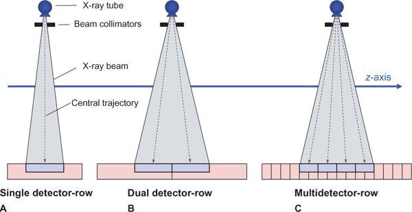
FIGURE 1-2 Comparison of the detector geometry of single detector-row scanners, dual detector-row scanners, and multidetector-row scanners—in this case, with 4 detector rows. (From M. Prokop et al. Spiral and Multislice CT of the Body. Thieme Medical Publishers 2003, with permission.)
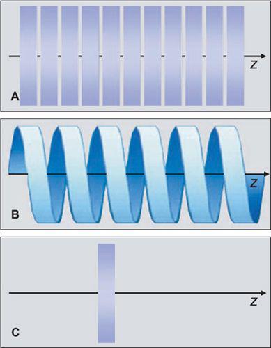
FIGURE 1-3 Principle of sequential scanning (A), spiral or helical scanning (B), and dynamic scanning (C). In sequential scanning, each section is acquired at a constant table position, then the table is moved and the next section is acquired. In spiral scanning, the table is moved during the acquisition process. In dynamic scanning, a particular section is scanned multiple times to evaluate temporal changes.
Sequential, spiral, or dynamic data acquisition is available with single detector-row as well as with multidetectorrow scanners.
SCANNING PARAMETERS
The most important scanning parameters for CT angiography are summarized in Table 1-1.
Acquisition Parameters
The following parameters described in Table 1-1 determine data acquisition:
• Number of active detector rows (N)
• Section collimation (SC)
• Rotation time (RT)
• Table feed per rotation (TF)
• Pitch factor (P): P = TF/(N × C
• Scan length (L)
• Tube voltage (U), also called the kVp setting
• Tube load (I × t), also called the mAs setting.
The number of active detector rows or simultaneously acquired sections is one for single detector-row CT, two for dual detector-row CT, and 4 to (presently 128 for multidetectorrow CT. Section collimation is determined by the total width of the acquired volume in the center of the scan field divided by the number of sections. The rotation time is the time it takes for the tube–detector unit to rotate once around the patient.
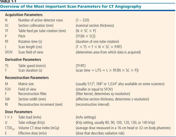
Table feed per rotation and pitch are parameters that are relevant for spiral scanning: The table feed indicates how much the table moves during the rotation time. The pitch factor provides the relation between table feed and total width of the acquired volume. The maximum pitch depends on the scanner manufacturer and usually varies between 1.5 and 2. For sequential scanning, the table feed between consecutive sections is usually chosen identical to the section collimation, and the resulting pitch is 1.
Scan length depends on the clinical indication. Scan duration can be derived from scan length and table speed, and thus the other parameters as described in Table 1-1.
Tube load, pitch, and tube voltage are main determinants of patient dose. Tube load, also called the mAs setting, is proportional to the radiation dose, while pitch is inversely proportional to it. This has led to the definition of effective tube load (or effective mAs: mAseff = mAs/P. Tube voltage (kVp setting determines the energy of the x-ray beam: At higher energy, there is more penetrating power. However, the x-ray attenuation of elements with a higher atomic number than water (for example, calcium or iodine will be relatively higher at lower x-ray energy. At constant mAs, the dose decreases if lower kVp settings are chosen.
Reconstruction Parameters
Image reconstruction is influenced by the following parameters (Table 1-1):
• Field of view (FOV)
• Matrix size (M)
• Reconstruction filter (F)
• Raw data interpolation algorithm (for spiral scanning)
• Reconstructed section width (SW, also called section thickness)
• Reconstruction increment (RI)
Image reconstruction starts with choice of a reconstruction field of view that determines which part of the data will end up in the images. The FOV is usually chosen from reference images that include the whole body cross sections and allows focusing on the region of interest. The matrix size of the reconstructed image usually is 5122, but modern scanners allow for other matrices as well (7682 or 1,024)2.
The reconstruction filter is required to reconstruct usable images from the projectional raw data. It determines the trade-off between spatial resolution in the imaging plane (xy-plane and the image noise. The raw data interpolation algorithm is necessary in spiral scanning to compensate for the continuous motion during the scan, but more sophisticated raw data interpolation algorithms are also used to compensate for cone beam effects in multidetector-row CT (p. 20).
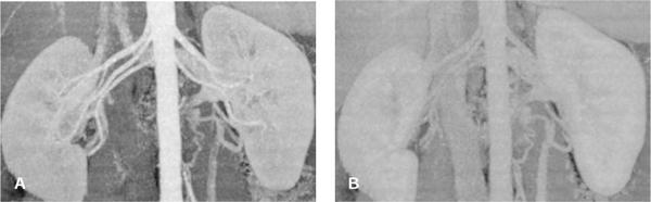
FIGURE 1-4 Contrast-to-noise ratio and image quality. Maximum intensity projection (MIP) of the renal arteries with high CNR in the arterial phase (A) and low CNR in the portal venous phase (B). Note that image noise and exposure parameters were similar in both examples, but the contrast enhancement was lower in the portal venous phase. In such a late phase, vessels can no longer be visualized if their enhancement is similar to that of the background tissue.
Reconstructed section width or section thickness refers to the thickness of the CT sections in the final images. In sequential scanning, section width and section collimation are identical. With spiral scanning, section width is commonly larger than section collimation (p. 13). With multidetectorrow CT, section width can be varied almost arbitrarily but is always larger than or equal to the chosen section collimation (p. 14). Section collimation therefore determines the thinnest section width that can be reconstructed.
The reconstruction increment is a parameter for spiral scanning: Here, images can be reconstructed at arbitrary increments that are smaller than the chosen section width or section collimation. In sequential scanning, the reconstruction increment is identical to the table feed between sections.
PERFORMANCE PARAMETERS
In order to be able to optimize image quality for CTA, it is helpful to understand the basic physical parameters that determine performance of a CT scanner or a scanning protocol. The main parameters are contrast-to-noise ratio and spatial resolution, which determine how well a vessel is displayed and how small a detail can be evaluated.
Contrast-to-Noise Ratio
The contrast-to-noise ratio (CNR) determines how well a given vessel can be displayed. At a high CNR, even small vessels can be detected, and vessel contours on 3D displays appear well defined (Fig. 1-4A). At a low CNR, small vessels may no longer be sufficiently visualized to make a diagnosis, and 3D displays of larger vessels may be irregular with insufficiently defined contours (Fig. 1-4B).
CNR is determined by the difference in CT numbers between vessel of interest and surrounding soft tissues in relation to the image noise:
CNR = (CTvessel − CTsoft tissue)/Noise
Contrast
The contrast in the CNR is determined by the enhancement of the target vessel and the CT number of the surrounding soft tissues. Since a vessel is rarely surrounded by only one type of soft tissue, CNR varies locally and may be difficult to determine in clinical practice. For this reason, water is frequently used as a substitute for soft tissue in the equation above.
To understand how the contrast is influenced by CT numbers, it is useful to have a quick look at CT-number definition: CT numbers are derived from the local x-ray attenuation (μ) by normalizing x-ray attenuation to water: CT = 1,000 × (μ − μwater)/μwater. The numbers are set on a scale in which −1,000 represents the attenuation of air and 0 is the attenuation of water. Note that there is no upper limit to the scale. In honor of Sir Godfrey N. Hounsfield, the inventor of CT, the unit for CT numbers is called the Hounsfield unit (HU. The normalization process reduces the dependence of the CT number on the energy of the radiation as long as the chemical composition of the examined structure is similar to that of water. This holds true for most soft tissues but is not the case for calcium or iodine-containing structures. Optimizing the energy of the x-ray beam therefore can be used to increase the CT numbers of contrast-enhanced vessels.
Enhancement of the target vessel depends on the local intravascular iodine concentration. This local iodine concentration is heavily influenced by the contrast material injection protocol (see Chapter 2 as well as by the timing of the scan. Intravenously injected contrast material first travels through the right heart and pulmonary system; then through the left heart, the aorta, and the arterial system; and finally returns back to the right heart via portal and systemic veins. Proper timing, depending on the target vessels, is therefore mandatory.
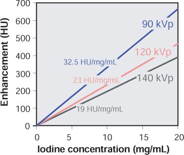
FIGURE 1-5 Vascular enhancement versus iodine concentration for various kVp settings. Note that enhancement per mg iodine is higher at lower kVp settings.
Enhancement is not only dependent on the local iodine concentration but also on the energy spectrum of the radiation. Within the energy range used for CT examinations, the CT numbers of iodine-containing contrast material increase rapidly as lower tube voltages (kVp settings are applied (Fig. 1-5). At identical intravascular iodine concentrations, better enhancement and therefore better contrast can be obtained at low kVp settings.
In clinical practice, surrounding tissues may also enhance. This is especially the case for parenchymal organs such as the liver or the kidneys. If such vessels are to be evaluated, the scan must be timed early enough to ensure that there is no substantial tissue enhancement present (compare Fig. 1-4).
Image Noise
Image noise refers to random variations in CT numbers, which cause problems in contour definition and low-contrast resolution (Fig. 1-6). Noise is mainly due to the limited amount of quanta that hit the CT detector array (quantum noise), but it is also caused by other sources such as the detector electronics (electronic noise). Image noise is usually described by the standard deviation of the CT numbers within a homogenous region of an object. Image noise is determined by the following factors:
• Radiation dose and quantum statistics (in principle, the number of photons that pass through the reconstructed voxel,
• Overall detector efficiency (the ability to detect as many quanta as possible and add as little additional noise from electronic detector components,
• Image interpolation (for example, to correct for motion in the case of spiral scanning, and
• Image reconstruction algorithm (the filter kernel that determines spatial resolution in the scan plane.
High image noise causes similar problems as low contrast: at high noise, small vessels may vanish, and contours are no longer sharply defined (Fig. 1-6).
Windowing
Windowing is a technique used in most imaging systems: It assigns only a small portion (window) on the number scale to actual gray levels that are displayed on a monitor or printed on film. Windowing is used to vary the visual contrast and brightness of a digital image. A window is characterized by its center (also called level) and its width.
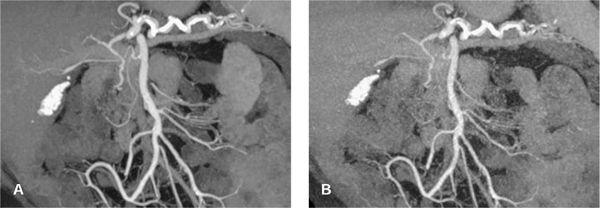
FIGURE 1-6 CTA angiography of a patient with an aberrant right hepatic artery arising from the superior mesenteric artery. The scan was part of an ECG-gated exam with 64 × 0.625 mm collimation acquired with 300 mAs (CTDIvol = 18 mGy). The untagged reconstruction takes advantage of all data and has a low image noise (A), while the gated reconstruction uses only about 15% of the data and therefore suffers from increased image noise (B). The periphery of the hepatic artery can no longer be evaluated in (B). Note that calcified gallstones also are displayed on these maximum intensity projections.
FIGURE 1-7 Effect of windowing. A narrow window enhances contrast and visual noise perception (A), while a wide window reduces contrast and noise perception (B). CNR is not affected. The window has to be wide enough that structures in enhanced lumen can be discerned. It has to be increased in width for vessels with higher enhancement.
Windowing affects visual contrast and noise perception equally. The contrast-to-noise ratio of the image is not affected. A wide window results in low contrast and little noise; a narrow window results in a high contrast but also a high noise (Fig. 1-7).
In practice, the optimum window width for CTA is determined by the intravascular contrast enhancement and, to a lesser degree, by the presence of wall calcifications or differences in tissues around the vessels. High enhancement and the presence of calcifications require a wide window, while insufficient enhancement requires narrower window settings. It is obvious that a high enhancement is desirable because it increases CNR and allows for using wider window settings that suppress image noise.
Spatial Resolution
Spatial resolution determines how small a detail can be evaluated and how sharp a given structure is depicted. Spatial resolution in a CT image depends on matrix size and system resolution. System resolution is determined by the scanner geometry and the chosen acquisition parameters. If the matrix is fine enough (small enough pixels, or picture elements, the spatial resolution in the image equals the system resolution. Commonly, the spatial resolution of an imaging system is described in one of the following three ways.
• The modulation transfer function (MTF) describes how much percent of its original contrast a structural detail of a certain size retains in the image (Fig. 1-8). The size of structural details is given in terms of spatial frequencies. The MTF is the most abstract and correct way of describing spatial resolution. The MTF decreases toward higher spatial frequencies. Vendors usually use a cutoff point around 4% and provide the corresponding spatial frequency (in cycles per centimeter as the maximum spatial resolution of the imaging system. However, a cutoff point of 4% has little to do with clinical reality. It means that the contrast of the original structure has been reduced by a factor of 25: For a small vessel, that will mean that its original contrast—for example, 500 HU—will have been reduced to 20 HU in the image. A cutoff frequency of 20% is much more realistic, but data at this point are less readily available (Fig. 1-8).
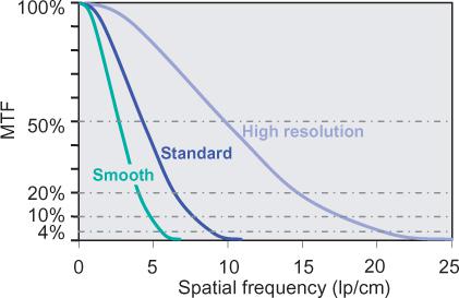
FIGURE 1-8 The modulation transfer function (MTF) describes how the contrast of a detail of a certain size (spatial frequency in line pairs per centimeter) is displayed in an image. In technical reports of scanner systems, spatial resolution is usually described as the spatial frequency at which the MTF reaches 4%. This value is unrealistic for CTA. A cutoff value of 20% or the mean of the cutoff values at 10% and 50% describe the systems better. In this example, MTFs for typical smooth, standard, and high resolution filters are provided. In CTA, only smooth and standard filters are used.
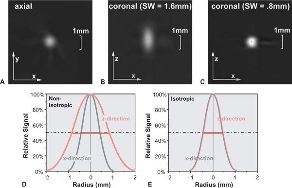
FIGURE 1-9 The point spread function (PSF) describes how a tiny detail is displayed in the image. Compare the images of a tiny gold bead in the axial plane (A) and the coronal plane scanned with a section width of 1.6 mm (B) and 0.8 mm (C). The CT number profile though the center of the bead corresponds to the PSF. In case of a section width of 1.6 mm, the PSFs in the x-direction and z-direction will differ (D), while for a section width of 0.8 mm, the PSFs in both directions are equal (E). Note that the width at 50% of the height of the PSF (full width at half maximum) is a good indicator of spatial resolution. (From M. Prokop et al. Spiral and Multislice CT of the Body. Thieme Medical Publishers 2003, with permission.)
• The full width at half maximum (FWHM) of the point spread function (PSF): The PSF describes how much every detail in an object gets blurred once it is displayed in an image (Fig. 1-9). Hence, the PSF is measured experimentally by imaging a very tiny detail that is substantially below the spatial resolution of the imaging system but that has a very high contrast. In practice, gold spheres or tungsten wires are used for this purpose. The width of the point spread function indicates the spatial resolution of the system: The smaller it is, the better the resolution. It is commonly used in the z-direction and is then called section width or effective section thickness (see also Fig. 1-14. In the xy-plane, it is probably the best way of comparing spatial resolution as well, but so far, it is not yet commonly provided by the manufacturers. An approximate relation to the MTF is provided in Table 1-2.
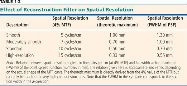
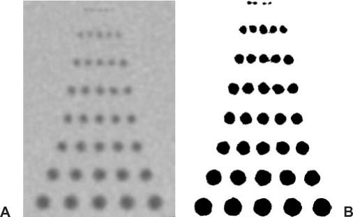
FIGURE 1-10 (A) Spatial resolution as indicated by groups of equidistant drill holes in Plexiglas measured with 64 × 0.625-mm section collimation. (B) Note that using a very narrow window setting can influence detail visibility.
• The smallest size of a group of equidistant lines or holes (Fig. 1-10): This way of displaying spatial resolution is the one that seems most intuitive, but it is also the one that is most prone to manipulation. By using very high contrast (e.g., air-filled holes or an aluminum grid to create lines) and then using a very narrow window setting (almost black and white), favorable results can be achieved that have little to do with clinical reality.
Matrix Size
Matrix size works as a limiting factor for spatial resolution. Too small a matrix can reduce spatial resolution, but a very large matrix size cannot increase resolution beyond the system resolution (Fig. 1-11). To be more precise, it is not the matrix size in itself but the resulting size of a single picture element (called a pixel) that limits spatial resolution. According to the sampling theorem, the pixel size should be at least one half the spatial resolution—as defined by the FWHM of the point spread function. In practice, further improvement in image quality can be seen if pixels are one third of the spatial resolution. Beyond that, the added value of even smaller pixel sizes is very limited.
Pixel size (p) is determined by the field of view (FOV) and the matrix size (M): p = FOV/M. In the imaging plane (xy-plane), the size of the reconstruction matrix is usually 5122, but newer scanners allow for 7682 and 1,0242 as well. For a full body cross section in the chest or abdomen, a FOV between 300 and 400 mm is required. The resulting pixel sizes vary from 0.6 to 0.8 mm if a 512 matrix is used.
In a coronal or sagittal plane derived from a 3D-image data set, the pixel size is derived from the pixel size in the xy-plane and by the reconstruction increment in the direction of the patient axis (z-direction). This reconstruction increment (RI) describes the distance between the centers of consecutive sections that are reconstructed from the CT raw data. In such coronal or sagittal planes, matrix size is no longer square but rectangular: In the x– or y-direction, it remains 512 (or higher, depending on the chosen reconstruction matrix, but in the z-direction, it is defined by the scan length (L and the reconstruction increment (RI): Mz = L/RI. Again, the pixel size in the z-direction (i.e., the RI) should be at least one half the spatial resolution in this direction. Spatial resolution in the z-direction is defined by the reconstructed section width (SW, see below “z-resolution”). For CT angiography, RI should therefore be not larger than SW/2.
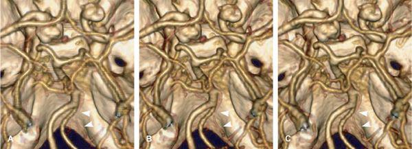
FIGURE 1-11 Effect of field of view (FOV) on spatial resolution. Volume-rendered images of the circle of Willis reconstructed with 40-cm FOV (A), 20-cm FOV (B), and 10-cm FOV (C), each with a 5122 matrix. The images were enlarged to yield the same details. While too large a FOV reduces quality, excessive reduction of FOV does not further improve it.
FIGURE 1-12 Comparison of image quality in an anisotropic data set (SW = 3 mm, RI = 1.5 mm) (A) and an isotropic reconstruction of the same data set (SW = 0.9 mm, RI = 0.5 mm) (B). Reconstructing even thinner sections leads to no further improvement (SW = 0.67 mm, RI = 0.35 mm) (C).
Taking the concept of pixel from 2D to 3D leads to volume elements (called voxels) that are defined by the pixel size in the xy-plane and the reconstruction increment in the z-direction. In most traditional CT examinations, the voxel has a matchstick shape, that is, the pixel size measured in the xy-plane is 5 to 10 times smaller than the reconstruction increment. For CTA, however, the pixel size in the xy-plane and the z-direction should be adapted to the available spatial resolution. For multidetector-row CT scanners, scan parameters should be chosen so that spatial resolution in the xy-plane is similar to resolution in the z-direction (isotropic resolution), and the voxels should also be isotropic (i.e., have a cubic shape). For this purpose, the reconstruction increment should be chosen similar to the pixel size (Fig. 1-12). With the newest generations of multidetector-row CT scanners, spatial resolution can now be higher in the z-direction than in the xy-plane, but choosing such parameters makes little sense for most indications (Fig. 1-12C).
xy-Resolution
Spatial resolution in the imaging plane (xy-plane is determined by the reconstruction filter (filter kernel used for the mathematical process of reconstructing transaxial cross-sectional images from projection data. The filter kernel determines the trade-off between spatial resolution and image noise (Fig. 1-13). The maximum spatial resolution that can be created with such filter kernels depends on the scanner geometry and increases, for example, for smaller detector elements or techniques such as quarter detector offset or flying focal spot. In CT angiography, image noise becomes a limiting factor. Moderately smoothing filter kernels are therefore preferred for most applications.
The xy-resolution is commonly given in line pairs per centimeter at the 4% value of the MTF. For practical purposes, however, the width of the point spread function yields numbers that can be better used to optimize scan and reconstruction parameters. Table 1-2 provides an overview of how these numbers relate.
z-Axis Resolution
The z-axis resolution is determined by the section width, the thickness of the reconstructed CT section. The section width is defined as the full width at half maximum (FWHM) of the section sensitivity profile, which shows how much a point in the object contributes to the image as a function of its distance from the center of the section (Fig. 1-14). Speaking in the terms defined earlier, the section profile is nothing other than the point spread function in the z-direction, while the section width is the FWHM of this point spread function.
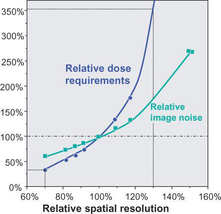
FIGURE 1-13 Spatial resolution versus image noise and dose requirements for constant SNR. Note that reduction in spatial resolution by 30% compared with standard filter kernel requires less than 50% of the dose for identical SNR, while increase in resolution by 30% requires a more than 2.5 times increase in dose. (From M. Prokop et al. Spiral and Multislice CT of the Body. Thieme Medical Publishers 2003, with permission.)
In sequential single detector-row CT scanning, section width and section collimation are identical. In fact, section collimation is defined as the FWHM of the section profile in the center of the scan field during a single scan without table movement. Under these conditions, the section profile approaches an “ideal” rectangular shape: Only points within a parallel section in the scanned object contribute to the image. In reality, the finite width of the focal spot of the x-ray tube, the cone shape of the x-ray beam, and other factors contribute to the fact that realistic section profiles are more rounded (Fig. 1-14A–C).
With the introduction of single detector-row spiral scanning, the section profile becomes bell-shaped (Fig. 1-14E). This is due to the interpolation that takes place in order to compensate for the table movement during the scan (p. 21). Depending on the pitch factor and the spiral interpolation algorithm, the section width increases by as much as 30% over the section collimation. Manufacturers differ in how they indicate the section width on their scan interface: Only Philips provides SW, all others provide SC, from which the user must calculate SW, depending on the pitch.
With multidetector-row CT, the section width becomes independent of the section collimation. The only precondition is that SW is larger than or equal to SC. This means that spatial resolution in the z-direction can easily be reduced if thin collimation had been chosen to scan the patient, but choosing too thick a collimation for scanning will not allow for improving z-axis resolution after the scan has been acquired. The various manufacturers have taken different approaches to the practical implementation of this principle: Some allow for continuous choice of SW, others allow for multiples of the chosen section width.
Temporal Resolution
Temporal resolution is described by the temporal acquisition window, the time period from which data are sampled to reconstruct an image. If raw data are weighted before reconstruction, the temporal resolution is frequently defined in analogy to spatial resolution as the full width at half maximum of the temporal weighting function.
SCANNER TECHNOLOGY
Detector Technology
Single detector-row scanners use a single detector arc or detector ring that consists of parallel detector elements that are much smaller in the direction of the arc (xy-plane) than in the z-direction (Fig. 1-2A). In fact, the detector elements are wide enough in the z-direction to accommodate the maximum section collimation (usually 10 mm) that is available on such scanners.
Dual detector-row scanners are based on a detector array that is twice as wide as a conventional CT detector and is split in half (Fig. 1-2B). These scanners became available in early 1992, but in 1998, the introduction of 4-detector-row scanners brought a technological breakthrough.
In multidetector-row CT, each element on the detector array is subdivided along the z-axis (Fig. 1-2C). These parallel detector rows can be electronically combined to yield between 4 and 128 separate sections per rotation, depending on the type of scanner (1–3). With the exception of most 64- and 128-detector-row scanners, the actual number of detector rows is much larger than the number of active detector rows (channels) in order to accomplish more than one collimation setting. Different collimation settings are achieved by adding the signals of neighboring detector rows.
While there were three distinct types of detector arrays with 4- to 8-detector-row scanners—namely matrix arrays, hybrid arrays, and adaptive arrays (Fig. 1-15)—10- to 16- detector-row scanners use only hybrid arrays, and 32- to 64-detector-row scanners use hybrid or matrix arrays. Matrix arrays consist of detector rows of identical thickness; hybrid arrays have a central group of detector rows whose thickness is half the thickness of the outer detector rows; while adaptive arrays have detector rows that get wider the more peripherally they are located.
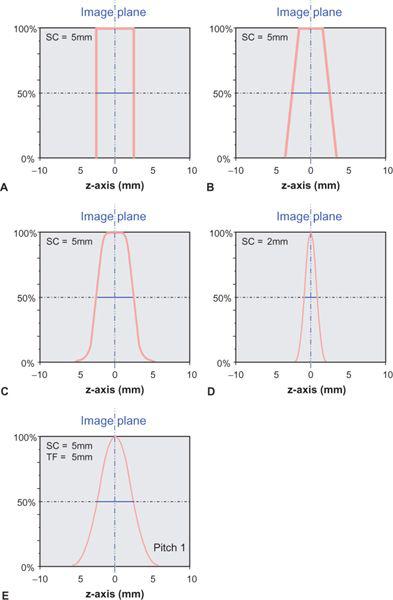
FIGURE 1-14 The section sensitivity profile (SSP) describes how much a point in the object contributes to the image as a function of its distance from the center of the section. Its full width at half maximum (FWHM) is called the section width or effective section thickness. Ideally, an SSP from a single scan (no table movement during data acquisition) should be rectangular (A). The penumbra, caused by the finite size of the focal spot of the x-ray tube, results in a more trapezoid shape of the SSP (B). Because of scatter within the object and other factors, a realistic SSP is more rounded (C). For thinner collimation, it even assumes a bell-shaped form (D). With spiral acquisition, the SSP is bell-shaped even for larger sections (E).
All 4- to 16-detector-row scanners provide multiple collimator settings with the maximum number of detector rows (Table 1-3). For hybrid and matrix arrays, the available section collimations are multiples of the thinnest detector width (Fig. 1-16A–B). For adaptive array detectors, the available section collimations are gained by combining signals from one, two, or more parallel rows with appropriate collimator settings (Fig. 1-16C). Most 64- and 128-detector-row scanners, however, do no longer provide the maximum number of sections for the largest available collimation (Fig. 1-17A–B). These scanners use matrix detector arrays of between 64 × 0.5 mm (128 × 0.5 mm) and 64 × 0.625 mm width. In these arrays, all 64 to 128 detector rows are read out simultaneously. As a consequence, only half the number of sections are available if the next wider collimation settings are chosen.
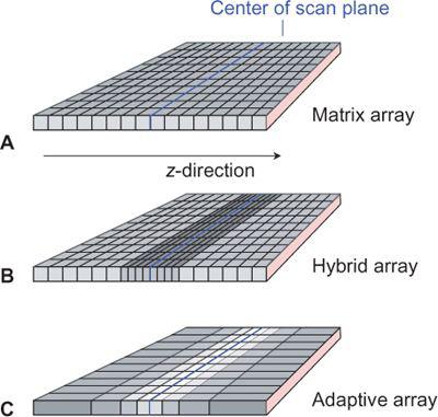
FIGURE 1-15 Detector configurations for multidetector-row CT: matrix array, in which all detector elements are equal (A); hybrid array, in which the innermost detectors are smaller (B); and adaptive array, in which the size detector rows increase with the distance from the center of the scan plane (C). Various section collimations can be created by proper collimation and combination of detector rows.
The only exception to this rule is a scanner that uses 32 active detector rows and z-flying focal spot technology (Fig. 1-17C). This scanner has a hybrid array that allows for section collimation of 32 × 0.6 mm and 20 × 1.2 mm. While this scanner actually provides a maximum of 32 sections per rotation (in the nonspiral, or sequence, mode, the manufacturer has opted for calling it a 64-slice scanner because the z-flying focal spot technology effectively doubles the data points (and thus the simultaneously acquired slices along the patient axis without having to increase the number of detector rows.
Flying Focal Spot Technology
Flying focal spot (FFS) technology refers to the position of the focal spot of the x-ray tube. The focal spot varies very rapidly between various positions on the anode, thus creating slightly different views of the object despite an (almost) identical position of the detector. The technology can be used to increase the number of x-ray projections for image reconstruction and, that way, allows for improving the spatial resolution of a scanner without creating “aliasing artifacts.” The technology is not new. It has been used for years to increase the number of projections within the imaging plane (xy-plane).
Recently, an additional movement along the z-axis (z-FFS was introduced that allows for increasing the number of projections also in the z-direction. The idea behind the technology is as follows. For image reconstruction, it is irrelevant whether projections from the tube to the detector or in the opposite direction, from the detector to the tube, are considered. This knowledge has been used for more than a decade for 180-degree interpolation algorithms in spiral CT, in which projection data from a conjugated spiral trajectory (detector to tube) are used for interpolation. Similarly, it can also be used for z-flying focal spot techniques (Fig. 1-18A): The linear trajectories from the tube to the centers of adjacent detector elements are identical to the trajectories from a single detector to multiple positions of the focal spot. However, there is a marked difference in the actual regions within the scanned object that are “seen” along each trajectory using these two techniques. In case of separate detector rows, these regions do not overlap, while they markedly overlap in the case of multiple focal spots (Fig. 1-18B). Currently, z-FFS technology is implemented in a way that two overlapping sections are irradiated, which are exactly 50% offset in the scan center. These sections converge (i.e., become identical) toward the detector and diverge (i.e., become separate)xs toward the tube with its flying focal spot (Fig. 1-18C). One has to keep in mind that despite the fact that the projections overlap in the center of rotation (by 0.3 mm), the thinnest available section width that can be reconstructed with z-FFS technology remains identical to the collimation (i.e., 0.6 mm).
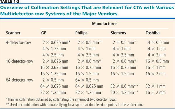
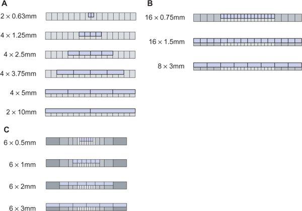
FIGURE 1-16 Various section collimations can be created by proper collimation and combination of detector rows. Example of a 4-detector-row scanner with matrix array (A), a 16- detector-row scanner with hybrid array (B), and a 6-detector-row scanner with adaptive array (C). (From M. Prokop et al. Spiral and Multislice CT of the Body. Thieme Medical Publishers 2003, with permission.)
Because the z-flying focal spot technology provides twice the data points in the z-direction over conventional technology with a single focal spot, aliasing artifacts in the z-direction are markedly reduced, even at higher pitch values (4). This is especially apparent for CTA images of the skull base and posterior fossa. If the number of projections is increased with conventional technology, however, similar artifact suppression can be reached. This requires low pitch factors or increasing the reconstructed section width by at least 30% over the chosen collimation (Fig. 1-19). For this reason, z-FFS yields the biggest advantages whenever very thin sections have to be reconstructed or high pitch factors have to be used.
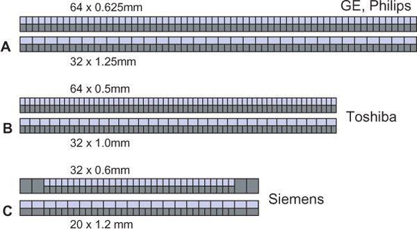
FIGURE 1-17 Comparison of various 64-slice detector configurations. GE and Philips use the same basic configuration with 64 × 0.625-mm and 32 × 1.25-mm collimation (A). Toshiba uses a 64 × 0.5-mm and 32 × 1.0-mm configuration (B). Siemens opted for a 32 × 0.6-mm and 20 × 1.2-mm configuration combined with z-flying focal spot technology (C). (From M. Prokop et al. Spiral and Multislice CT of the Body. Thieme Medical Publishers 2003, with permission.)

FIGURE 1-18 Principles of z-flying focal spot technology (z-FFS). The number of projection data can be increased if multiple detector elements or multiple focal spots are used: The central x-ray trajectories from the tube to multiple detector elements are identical to the trajectories from multiple tube positions (or focal spots) to a singledetector element (A). If not only the central line of the trajectory but also the width of the beam is considered, however, it becomes apparent that the sampled data is not identical. While the beams do not overlap in the case of multiple detector rows, the beams overlap to a varying degree in case of multiple focal spots (B). In the center of the scan field, a 50% overlap between beams can be created if only two focal spots are used (C). In the periphery of the scan field, gaps between the two beams occur close to the tube, while there is a higher overlap close to the detector.
Finally, it has to be noted that the number of focal spots plays no role for the calculation of pitch factors or other crucial scanner characteristics. A scanner with 32 active detector rows and 2 focal spots will therefore behave like a 32-detector-row scanner and not like a 64-detectorrow scanner when it comes to pitch, scanning speed, or even detector width. To mark this difference, it might be useful to distinguish between detector rows on the one hand and slices on the other: A 64-slice scanner that employs two z-flying focal spots should therefore correctly be addressed as a 32-detector-row scanner with dual z-FFS technology. The technique holds a lot of promise, and in the future, tubes with multiple focal spots can be expected.
Dual Source Technology
Multiple source technology refers to scanners with more than one tube–detector array combination (5). They are primarily being developed for cardiac CT. Presently, dual source scanners are becoming available that have the advantage that the time required to acquire data for one image is cut in half by the two acquisition systems. Another potential advantage is the availability of a dual energy technique: The two tubes can operate at different kVp settings, and the differences in x-ray absorption at identical projection angles can be used to separately display materials of differing atomic number, such as calcium, iodine, or soft tissues. It remains to be seen whether the ultimate goal of reducing the negative influence of vessel wall calcifications in coronary CTA can be reached.
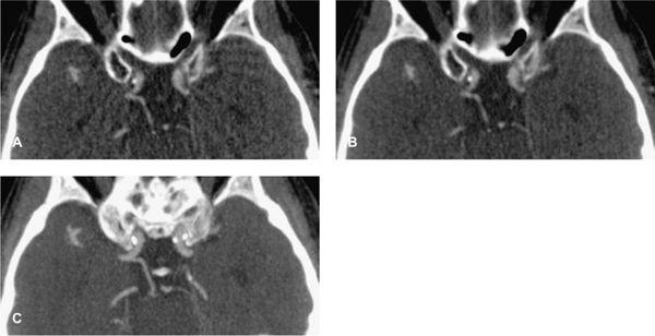
FIGURE 1-19 Aliasing artifacts occur mainly in regions with rapid transitions in x-ray attenuation along the z-axis, such as the posterior fossa (A). The artifacts are worse if the thinnest possible section thickness is reconstructed (here, 0.67-mm-thick sections acquired with 64 × 0.625-mm collimation) but decrease substantially if a >30% wider section thickness (0.9-mm-thick sections reconstructed from the same raw data set) is chosen (B). Using a z-flying focal spot, the amount of aliasing at 0.6-mm-thick sections can be expected to be similar to (B). Independent of the aliasing artifacts, however, diagnosis of a hypoplasic posterior communicating artery (arrow) can be made from 4-mmwide thin-slab MIP based on the 0.67-mm-thick image data set (C).
In dual source scanners, one of the detector arrays has a normal size (in xy-direction) to be able to perform standard CT examinations. The second detector array is narrower because it only is used for cardiac examinations (Fig. 1-20). The effective rotation time is reduced from 330 ms for a single source scanner to 165 ms for a dual source scanner. Maximum temporal resolution with these scanners is below 90 ms.
Scanner Performance
The most important factor that determines scanner performance for CTA is the relation between scanning speed and z-resolution. This performance parameter can be defined as the ratio between maximum table speed and thinnest section width that can be reconstructed using that table speed. Scanner performance, when defined that way, has been doubling approximately every 2 years since the mid 1980s (Fig. 1-21). As compared to 4-detector-row scanners, performance of 32- to 64-detector-row scanners has increased more than 20 times owing to more detector rows and faster rotation speed.
This increase in performance made it possible to acquire isotropic data and even reduce scan duration with multidetector-row scanners. While spiral CT scanning with single detector-row scanners made it possible to perform thoracic or abdominal CTA during a single breath-hold phase of approximately 30s, the advent of 4-detector-row scanners made it possible to acquire the data in a near isotropic fashion. With 16-detector-row scanners, nearisotropic resolution could be combined with sub-mm resolution and scan durations of between 8 and 15s for chest or abdomen (Table 1-6) (6). With 32- to 128-detector-row scanners, scan duration can always be kept well below 10s, even for submillimeter resolution. However, this decrease in scan duration may not always be advantageous: Especially for large aneurysms or vessel occlusions, it takes longer to completely enhance the vessel of interest, and scanning too early or too fast will lead to suboptimum contrast enhancement (see also Fig. 1-31). For this reason, 16-detector-row units suffice for providing excellent spatial resolution and good handling for the vast majority of CTA examinations.
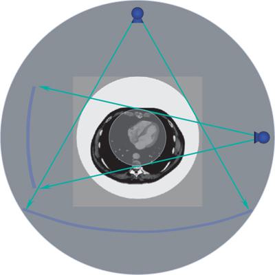
FIGURE 1-20 Principle of dual source technology: Two x-ray tubedetector arrays rotate simultaneously around the body, thus reducing effective rotation time, the time required to acquire a full 360-degrees of projectional data.
Related posts:

Stay updated, free articles. Join our Telegram channel

Full access? Get Clinical Tree


