Cranial CT: Normal Findings
The scan usually begins at the base of the skull and continues upward. Since the hard copies are oriented such that the sections are viewed from caudal, all structures appear as if they were left/right reversed (see p. 14). The small topogram shows you the corresponding position of each image.

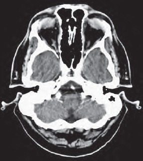


You should first check for any swellings in the soft tissues which may indicate trauma to the head. Always examine the condition of the basilar artery (90) in scans close to the base of the skull and the brainstem (107). The view is often limited by streaks of artifacts (3) radiating from the temporal bones (55b).
When examining trauma patients, remember to use the bone window to inspect the sphenoid bone (60), the zygomatic bone (56), and the calvaria (55) for fractures. In the caudal slices you can recognize basal parts of the temporal lobe (110) and the cerebellum (104).
Orbital structures are usually viewed in another scanning plane (see pp. 33–40). In Figure 27.1–3 we see only a partial slice of the upper parts of the globe (150), the extraocular muscles (47), and the olfactory bulb (142).


As the series of slices continues dorsally, the crista galli (162) and the basal parts of the frontal lobe (111) appear. The pons/ medulla (107) are often obscured by artifacts (3). The pituitary gland (146) and stalk (147) are seen between the upper border of the sphenoid sinus (73) and the clinoid process (163). Of the dural sinuses, the sigmoid sinus (103) can be readily identified. The basilar artery (90) and the superior cerebellar artery (95a) lie anterior to the pons (107). The cerebellar tentorium (131), which lies dorsal to the middle cerebral artery (91b), shouldn’t be mistaken for the posterior cerebral artery (91c) at the level depicted in Figure 29.1a on the next page. The inferior (temporal) horns of the lateral ventricles (133) as well as the 4th ventricle (135) can be identified in Figure 28.3 . Fluid occurring in the normally air-filled mastoid cells (62) or in the frontal sinus (76) may indicate a fracture (blood) or an infection (effusion). A small portion of the roof of the orbit (*) can still be seen in Figure 28.3 .


In Figures 28.3a and 29.1a partial volume effects of the orbit (*) or the petrosal bone (**) might also be misinterpreted as fresh hemorrhages in the frontal (111) or the temporal lobe (110).


The cortex next to the frontal bone (55a) often appears hyperdense compared to adjacent brain parenchyma, but this is an artifact due to beam-hard-ening effects of bone. Note that the choroid plexus (123) in the lateral ventricle (133) is enhanced after i.v. infusion of CM. Even in plain scans it may appear hyperdense because of calcifications.


You will soon have recognized that the CCT images on these pages were taken after i.v. administration of CM: the vessels of the circle of Willis are markedly enhanced. The branches (94) of the middle cerebral artery (91b) are visible in the Sylvian fissure (127). Even the pericallosal artery (93), a continuation of the anterior cerebral artery (91a), can be clearly identified. Nevertheless, it is often difficult to distinguish between the optic chiasm (145) and the pituitary stalk (147) because these structures have similar densities.


In addition to the above-mentioned cerebral arteries (93, 94), the falx cerebri (130) is a hyperdense structure. In Figure 30.2a you can see the extension of the hyperdense choroid plexus (123) through the foramen of Monro, which connects the lateral ventricles (133) with the 3rd ventricle (134). Check whether the contours of the lateral ventricles are symmetric.


A midline shift could be an indirect sign of edema. Calcifications in the pineal (148) gland and the choroid plexus (123) are a common finding in adults, and are generally without any pathologic significance. Due to partial volume effects, the upper parts of the tentorium (131) often appear without clear margins so that it becomes difficult to demarcate the cerebellar vermis (105) and hemispheres (104) from the occipital lobe (112).


It is particularly important to carefully inspect the internal capsule (121) and the basal ganglia: caudate nucleus (117), putamen (118), and globus pallidus (119) as well as the thal-amus (120). Consult the number codes in the front foldout for the other structures not specifically mentioned on these pages.


The position of the patient’s head is not always as straight as in our example. Even small inclinations may lead to remarkably asymmetric pictures of the ventricular system, though in reality it is perfectly normal. You may see only a partial slice of the convex contours of the lateral ventricles (133). This could give you the impression that they are not well defined ( Fig. 31.1a ).


The phenomenon must not be confused with brain edema: as long as the sulci (external SAS) are not effaced, but configured regularly, the presence of edema is rather improbable.


For evaluating the width of the SAS, the patient’s age is an important factor. Compare the images on pages 50 and 52 in this context. The paraventricular and supraventricular white matter (143) must be checked for poorly circumscribed hypodense regions of edema due to cerebral infarction.
As residues of older infarctions, cystic lesions may develop. In late stages they are well defined and show the same density as CSF (see p. 58).


In the upper sections ( Figs. 32.1–32.3 ) calcifications in the cerebral falx (130) often appear. You should differentiate this kind of lesion, which has no clinical significance, from calcified meningioma. The presence of CSF-filled sulci (132) in adults is an important finding with which to exclude brain edema. After a thorough evaluation of the cerebral soft-tissue window, a careful inspection of the bone window should follow. Continue to check for bone metastases or fracture lines. Only now is your evaluation of a cranial CT really complete.

Test yourself! Exercise 1:
Note from memory a systematic order for the evaluation of cranial CTs. If you have difficulties, return to the checklist on page 26.
Note: | • |
• | • |
• | • |
• | • |
• | • |


On the following pages the atlas of normal anatomy continues with scans of the orbits (axial), the face (coronal), and the petrosal bones (axial and coronal). After these you will find the most common anatomic variations, typical phenomena caused by partial volume effects and the most important intracranial pathologic changes on pages 50 to 60.
The face and the orbits are usually studied in thin slices (2 mm) using 2-mm collimation steps or even thinner. The orientation of the scanning plane is comparable to that for CCTs (see p. 26). In the sagittal topogram the line of reference lies parallel to the floor of the orbit at an angle of about 15° to horizontal ( Fig. 33.2 ).
The printouts are usually presented in the view from caudal: all structures on the right side of the body appear on the left, and vice versa.


Alterations in the soft structures of the orbits and the paranasal sinuses can be readily evaluated in the soft-tissue window ( Fig. 33.1b ). For the detection of a tumor-related erosion of bone or a fracture, the bone window should also be checked ( Fig. 33.1a ). The following pages therefore present each scan level in both windows. The accompanying drawing ( Fig. 33.1c ) refers to both. The number codes for all drawings are found in the legend in the front foldout.
On the lower slices of the orbits you will see parts of the maxillary sinus (75), the nasal cavity (77) with the conchae (166), the sphenoid sinus (73), and the mastoid cells (62) as air-filled spaces. If there is fluid or a soft-tissue mass, this may indicate a fracture, an infection, or a tumor of the paranasal sinuses. For examples of such diseases, see pages 58 to 61.
Two parts of the mandible appear on the left side: in addition to the coronoid process (58), the temporomandibular joint with the head of the mandible (58a) is seen on the left. The carotid artery, however, is often difficult to discern in the carotid canal (64), whether in the soft-tissue or bone window.
In the petrous part of the temporal bone (55b), the tympanic cavity (66) and the vestibular system are visible. For a more detailed evaluation of the semicircular canals and the cochlea, images obtained with the petrous bone technique are more appropriate (pp. 44–47). CM was infused intravenously before the examination of the orbits. The branches of both the facial and angular vessels (89) as well as the basilar artery (90) there-fore appear markedly hyperdense in the soft-tissue window ( Fig. 33.1b ).
It is not always possible to achieve a precise sagittal position of the head. Even a slight tilt ( Fig. 34.1 ) will make the temporal lobe (110) appear on one side, whereas on the other side the mastoid cells (62) can be seen.


As experience shows, it is difficult to determine the course of the internal carotid artery (85a) through the base of the skull and to demarcate the pterygopalatine fossa (79), through which, among other structures, the greater palatine nerve and the nasal branches of the pterygopalatine ganglion (from CN V and CN VII) pass.


On the floor of the orbit, the short inferior oblique muscle (47f) often seems poorly delineated from the lower lid. This is due to the similar densities of these structures. Directly in front of the clinoid process/dorsum sellae (163) lies the pituitary gland (146) in its fossa, which is laterally bordered by the carotid siphon (85a).


Small inclinations of the head cause slightly asymmetric views of the globe (150) and the extraocular muscles (47). The medial wall of the nasolacrimal duct (152) is often so thin that it cannot be differentiated. At first sight the appearance of the clinoid process (163), between the pituitary stalk (147) and the carotid siphon (85a) on the left side only, may be confusing in Figure 37.2b .


After intravenous injection of CM, the branches of the middle cerebral artery (91b) originating from the internal carotid artery (85a) are readily distinguished. The gray shade of the optic nerves (78) as they pass through the chiasm (145) to the optic tracts (144), however, is very similar to that of the surrounding CSF (132). You should always check on the symmetry of the extraocular muscles (47) in the retrobulbar fatty tissue (2).


In the globe (150) you can now see the hyperdense lens (150a). Notice the oblique course of the ophthalmic artery (*) crossing the optic nerve (78) in the retrobulbar fatty tissue (2). Figure 39.2b shows a slight swelling (7) of the right lacrimal gland (151) compared to the left one (see Fig. 40.1b ).


Figure 40.1b clarifies that in this case there is indeed an inflammation or tumor-like thickening (7) in the right lacrimal gland (151). The superior rectus muscle (47a) appears at the roof of the orbit and immediately next to it lies the levator palpebrae muscle (46). Due to similar densities, these muscles are not easily differentiated.


The axial views of the orbits and the face end here with the appearance of the frontal sinus (76). Examples of pathologic changes of the orbits or fractures of facial bones are found on pages 61 to 63.
The possibilites of angling the CT gantry are limited. In order to achieve scans in the coronal plane, the patients were formerly positioned as shown in the planning topogram ( Fig. 41.1 ) in a prone position with the head completely extended. Nowadays coronal images are reconstructed digitally, based upon the threedimensional data set with a narrow collimation in MDCT-units, so that especially trauma patients do not have to be excluded any more for potential lesions of bones or ligaments of their cervical spine. Usually, images are viewed from anterior: the anatomic structures on the patient`s right side appear on the left in the images and conversly, as if the examiner were facing the patient.
When looking for fractures, images are usually acquired in the thin-slice mode (slice and collimation, each 2 mm) and viewed on bone windows. Even fine fracture lines can then be detected. A suspected fracture of the zygomatic arch may require additional scans in the axial plane (see p. 34). In Figure 41.2a the inferior alveolar canal (*) in the mandible (58) and the foramen rotundum (**) in the sphenoid bone (60) are clearly visible. As for the previous chapter, the code numbers for the drawings are explained in the legend in the front foldout.


The insertions of the extraocular muscles on the globe (150) can also be clearly identified (47 a–f) in the anterior slices. The short inferior oblique muscle (47f), however, is often seen only in coronal scanning planes, because it does not pass with the others muscles through the retrobulbar fatty connective tissue. The same problem occurs in axial scans of the face (compare with Fig. 36.2b and Fig. 36.2c ).
If a case of chronic sinusitis is suspected, it is very important to check whether the semilunar hiatus is open. It represents the main channel for discharging secretions of the paranasal sinuses. In Figure 60.3 you will find examples of anatomic variations which narrow this channel and may promote chronic sinusitis.
Sometimes one discovers a congenitally reduced pneumatization of a frontal sinus (76) or an asymmetric arrangement of other paranasal sinuses without any pathologic consequences. You should always make sure that all paranasal sinuses are filled exclusively with air, that they are well defined and present no air-fluid levels. Hemorrhage into the paranasal sinuses or the detection of intracranial bubbles of air must be interpreted as an indirect sign of a fracture – you will find examples of such fractures on page 63.
Test Yourself!
On the previous pages you have learned about the normal anatomy of the brain, the orbits, and the face. It may be some time ago that you studied the technical basics of CT and about adequate preparation of the patient. Before going on with the anatomy of the temporal bone, it would be good to check on and refresh your knowledge of the last chapters. All exercises are numbered consecutively, beginning with the first one on page 32.
Without doubt, you will improve your understanding of the subject if you tackle the gaps in your knowledge instead of skipping problems or looking at the answers at the end of the book. Refer to the relevant pages only if you get stuck.
Exercise 2: Write down from memory the typical window parameters for images of the lungs, bones, and soft tissues. Note precisely the width and center of each window in HU and give reasons for the differences. If you have difficulties answering this question, go back to pages 16/17 to refresh your memory.
Lung-/pleura window: | Center | Width | Grey scale range |
|
|
| ______ HU to ______ HU |
Bone window |
|
|
|
|
|
| ______ HU to ______ HU |
Soft-tissue window |
|
|
|
|
|
| ______ HU to ______ HU |
Exercise 3: Which two types of oral CM do you know? What specific aspects must you consider when administering this kind of CM depending on the clinical problem? Are there any consequences for your list?
Oral CM (name) | Indication | Special schedule |
Exercise 4: What aspects should you always a) clarify before referring your patients to a CT examination which probably requires the i.v. infusion of CM? The same applies if you consider referring someone to avenogram/angiogramoran b) IVU (both procedures are carried out with nonionic CM containing iodine). MRI examinations, however, are carried out with gadolinium as the CM. (The answers to questions 3 and 4 can be found c) on pp. 18 and 19.)
Exercise 5: How would you differentiate between long structures such as vessels, nerves, or certain muscles and nodular structures such as lymph nodes or tumors? (You will find the answer on p. 15.)

Exercise 6: In which vessels might you find turbulence phenomena, caused by the CM injection, that must not be mistaken for a thrombus? (If you don’t remember, check back to pp. 21–23.)

Thin-section CT scans (ultra-high resolution CT or UHRCT) are generally used to visualize the petrous bone for evaluating the inner ear. This technique employs slice thicknesses of 0.3 to 1.0 mm with continuous advancement of the couch between successive slices. Better spatial resolution and detail enlargement are achieved by imaging only a reduced FOV in the petrous bone using the thin-section technique as opposed to imaging the entire head. The petrous bone (55 b) of each side is visualized separately at high magnification. From experience, this is the best way to visualize small anatomic structures such as the auditory apparatus (61 a-c), the cochlea (68), or the semicircular duct (70 a-c).
The scout topogram film ( Fig. 46.1 ) shows the coronal slices. It is no longer necessary to position the patient prone with the neck hyperextended (see p. 41). The larger tilting angle of the gantry in today’s CT systems makes it possible to obtain these slices even in a supine patient.
Note the pneumatization of the mastoid cells (62) and the normally thin wall of the external acoustic meatus (63 b). Inflammations in these air-filled spaces lead to characteristic effusions and/or mucosal thickening (see Fig. 60.2 a ).


Analogous to coronal images, axial images are obtained with thin slices without overlap, i.e., 2 mm thickness and 2 mm increment and viewed on bone windows. The cerebellar hemispheres (104), the temporal lobe (110), and the soft tissues of the galea are therefore barely identifiable. Apart from the ossicles (61a–c) and the semicircular canals (70a–c), the internal carotid artery (64), the cochlea (68), and the internal (63a) and external auditory canals (63b) are visualized. The funnel-shaped depression in the posterior rim of the petrosal bone ( Fig. 48.2a ) represents the opening of the perilymphatic duct (** = aqueduct of the cochlea) into the subarachnoid space. In Figure 49.1a note the localization of the geniculate ganglion of the facial nerve (*) ventral to the facial canal. The topogram ( Fig. 48.1 ) shows an axial plane of section, obtained with the patient lying supine.
Test Yourself! Exercise 7: Think about differential diagnoses involving effusion in the middle ear (66), the outer auditory canal, or the mastoid cells (62) and compare your results with the cases shown on pages 60 and 62 to 63.


Do you remember the systematic sequence for evaluating CCT scans? If not, please go back to the checklist on page 26 or to your own notes on page 32.
After evaluating the soft tissues it is essential to examine the inner and outer CSF spaces. The width of the ventricles and the surface SAS increases continuously with age.


Since the brain of a child ( Fig. 50.1a ) fills the cranium (55), the outer subarachnoid space is scarcely visible, but with increasing age the sulci enlarge ( Fig. 50.2a ) and CSF (132) becomes visible between cortex and calvaria. In some patients this physiologic decrease in cortex volume is especially obvious in the frontal lobe (111). The space between it and the frontal bone (55a) becomes quite large. This so-called frontally emphasized brain involution should not be mistaken for pathologic atrophy of the brain or congenital microcephalus. If the CT scan in Figure 50.1a had been taken of an elderly patient, one would have to consider diffuse cerebral edema with pathologically effaced gyri. Before making a diagnosis of cerebral edema or brain atrophy you should therefore always check on the age of the patient.


Figure 50.2a shows an additional variation from the norm. Especially in middle-aged female patients you will sometimes find hyperostosis of the frontal bone (55a) (Steward-Morel-Syndrome) without any pathologic significance. The frontal bone (55a) is internally thickened on both sides, sometimes with an undulating contour. In cases of doubt, the bone window can help to differentiate between normal spongiosa and malignant infiltration.


An incomplete fusion of the septum pellucidum (133a) can, as another variation, lead to the development of a so-called cavum of the septum pellucidum. Please review the normal scans in Figures 30.2a , 30.3a , and 31.1a for comparison. Usually only the part of the septum located between the two anterior horns of the lateral ventricles ( Fig. 51.1a ) is involved, less frequently the cavum extends all the way to the posterior horns ( Fig. 51.2a ).


In the plane of Figure 51.1 , just medial of the head of the caudate nucleus (117), you can evaluate both foramina of Monro (141) which function as a route for the choroid plexus (123) and the CSF from the lateral ventricles (133) to the 3rd ventricle (134). Refresh your anatomic skills by naming all other structures in Figure 51.1 and checking your results in the legend.


The radiologist will rarely be confronted with an eye prosthesis (*) after enucleation of a globe (150). In patients with a history of orbital tumor, a local relapse, i.e. in the retrobulbar space (2) has to be ruled out in check-up CT scans. The CT scan of the orbit in Figure 51.3a showed minor postoperative change without any evidence of recurrent tumor.
One of the most important rules of CT scan interpretation is to always compare several adjacent planes (see pp. 14–15). If the head is tilted even slightly during the scan procedure, one lateral ventricle (133) for example, can appear in the image plane (dS), whereas the contralateral ventricle is still outside the plane ( Fig. 52.1 ). Only its roof will appear.
The computer therefore calculates a blurred, hypodense area which could be mistaken for a cerebral infarction ( Fig. 52.2a ). By comparing this plane with the adjacent one below it ( Fig. 52.3a ), the situation becomes clear, since the asymmetric contours of the imaged ventricles are now obvious.


This example illustrates the importance of the correct placement of the patient’s head. The exact position of the nose in an a.p. projection is obtained by using the gantry positioning lights. Involuntary movements of the head can be kept at a minimum by soft padding. In ventilated or unconscious patients an additional immobilization of the head with suitable bandings may be necessary.
One of the first steps in interpreting CCTs is the inspection of the soft tissues. Contusions with subcutaneous hematomas (8) may indicate skull trauma ( Fig. 53.1a ) and call for a careful search for an intracranial hematoma. Many injured patients cannot be expected to have their heads fixed for the duration of the CT scan, and this leads to considerable rotation. Asymmetric contours (* in Fig. 53.1b ) of the roof of the orbit (55a), the sphenoid bone (60), or the petrosal bone (not asymmetric in the illustrated examples!) are therefore frequent occurrences and may lead to misinterpretations of the hyperdense bone as a fresh intracranial hematoma.


The question of whether it is just an asymmetric projection of the skull base or a real hematoma can be answered by comparing adjacent sections ( Fig. 53.2a ). In this example the bones of the skull base caused the hyperdense partial volume effect. Despite the obvious right frontal extracranial contusion, intracranial bleeding could not be confirmed. Please note the considerable beam hardening (bone) artifacts (3) overlapping the brain stem (107). Such artifacts would not appear in MR images of these levels.


Related posts:


Stay updated, free articles. Join our Telegram channel

Full access? Get Clinical Tree


