Data Space

Introduction

Before we can understand k-space, we need to discuss the data space, which is a matrix of the processed image data. To most radiologists, kspace is in the twilight zone! We have already seen some of the basic concepts of the data space and k-space in the previous chapters. In this chapter, we will learn some of the properties of k-space in greater detail. The understanding of k-space is crucial to the understanding of some of the newer MRI fast scanning techniques such as fast spinecho (FSE) and echo planar imaging (EPI).

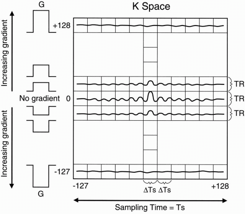Figure 13-1. The data space (with both axes as time variables) is an “analog” version of k-space.

Where Does k-Space Come From?

k-Space is derived from the data space, so it’s really not as intimidating as it initially appears. Figure 13-1 demonstrates a typical representation of the data space with a 256 × 256 matrix.

Figure 13-1 is an “analog” version of kspace. The true k-space, as we’ll see later, is a digitized version of this figure, with axes referred to as spatial frequencies.
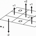
In Figure 13-1, we have 256 phase-encoding steps. We keep the zero-step (i.e., no
phase encoding) in the middle of k-space, so we go from −127 phase encode to +128 phase encode (bottom to top).
We also have 256 frequencies.
The y-axis, then, is the phase-encoding direction.
In the center, we put the signal acquired with no phase-encoding gradient.
As one advances on the y-axis, each set has signal acquired with an increasing phaseencoding gradient with maximum gradient at +128 phase-encoding step. Likewise, as one goes down from zero gradient in the y-axis, each step has signal acquired with an increasing phase-encoding gradient in the opposite direction with maximum gradient at −127 phase-encoding step.

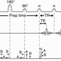
Let’s now go back and review the spin-echo pulse sequence (Fig. 13-2).

We apply the 90° pulse using an appropriate slice-select gradient, G_z.
Next, we apply a 180° pulse and, after a time, TE receives an echo.
During this time, we apply the readout gradient, G_x.
Then we place a sampled version of this echo in one of the rows in k-space. Let’s say that this echo was obtained without using a phase-encoding gradient in the y direction. We sample the signal and then put it into the zero line in the data space.
With, say, a 256 × 256 matrix, we take 256 samples. Each of the 256 points in a row of the data space is a sample of the echo. (It’s hard to draw discrete samples, so we’ll draw continuous signals in the data space rows, realizing that each point in a row is a digitized sample of the signal.)

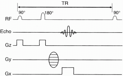
Figure 13-2. A spin-echo pulse sequence diagram.
For the second row in the data space, we do the exact same thing, except in this step the signal is obtained using a largar phaseencoding gradient in the y-axis.

Remember that the phase-encoding gradient causes dephasing of the signal. Therefore, the signal for the second line of the data space will be similar in shape to the first signal (because both are signals from the same slice of tissue, just obtained at a different time) but smaller in magnitude than the first signal (because it undergoes additional dephasing due to the phase-encoding gradient). Thus, when we draw this signal into the second line in the data space, we see that it is similar in shape to the first signal, but slightly weaker—because it’s been dephased.

The signal that goes into the last line of the data space (+128) will be almost flat because it has undergone maximum dephasing; likewise, as we alternate to the signals placed below the zero line (i.e., −1, −2, …, −127), a certain symmetry results. For instance, line (−1) is similar in strength to line (+1) in that, whereas line (+1) experiences mild dephasing due to a slight increase in magnetic field strength, line (−1) experiences similar mild dephasing due to a slight decrease in magnetic field strength. Likewise, the signal that goes into the first line in the data space (−127) will be almost flat due to maximum dephasing in the opposite direction of line (+128).

Remember that each line in the data space contains the signal obtained from the entire image slice during a single TR. Each TR is obtained using a different phase-encoding step in the y-axis.

Question 1: How long does it take to go from one row in the data space to another?

Answer: It takes the time of one TR.

Question 2: How long does it take to go from one point (sample) in a row to the next point (sample) in the same row of the data space?

Answer: It takes the time spent between samples, that is, the sampling interval (ΔT_s).

Question 3: How long does it take to fill one row of the data space?

Answer: Let’s say that ΔT_s [all equal to] 31 µsec and that there are 256 (N) samples along the readout axis. The sampling time is T_s = (ΔT_s)(N) = (31µsec)(256) = 7.9 msec

Therefore, it takes about 8 msec to fill one line of the data space. In general, it takes T_s = N_x · ΔT_s

to fill one line of the data space.

Question 4: How long does it take to fill one column of the data space?

Answer: It is the acquisition time N_p × TR, where N_p is the number of phase-encoding steps.

Let’s say TR = 3000 msec and N_p = 256.

Acquisition time = (3000 msec) (256)

= 12.8 min

If TR = 500 msec, then

Acquisition time = (500) (256) [all equal to] 2 min

It takes several milliseconds to fill one row of the data space. But it takes several minutes to fill the columns of the data space.

Motion Artifacts

The preceding concept is one of the reasons why motion artifacts manifest themselves mainly in the phase-encoding direction. In other words, it takes much longer to gather the signal in the phase-encoding direction than in the frequencyencoding direction, leaving more time for motion to affect the image in the phase direction. Another reason, as we shall see later, is that motion in any direction results in a phase change; thus, motion artifact propagates along the phase-encoding direction.

Properties of k-Space

Center of k-Space. The center of the data space contains maximum signal. This finding is caused by two factors:

Each of the signals has its maximum signal amplitude in the center column (Fig. 13-3). Recall that when we apply the 180° refocusing pulse, the dephased signal begins to rephase and reaches maximum amplitude when the protons are completely rephased. It then decreases in amplitude as the protons dephase once more.

The middle column in the data space corresponds to the center of each individual echo, and the more peripheral columns refer to the more peripheral segments of the echoes: columns to the left of center depict rephasing of the echoes toward maximal amplitude in the data space; columns to the right of center depict dephasing of the echoes away from maximal amplitude in the data space.

Therefore, as we go further out to the more peripheral columns, the signal weakens. The most peripheral points in the signal to the left are the weakest point of the signal as the signal just begins to rephase (Fig. 13-3). Likewise, the most peripheral point in the signal to the right is the weakest point after the signal has been refocused and then has regained maximum dephasing.
The maximum amplitude occurs in the center row because this line is obtained without additional dephasing due to phase-encoding gradients; subsequent rows with progressively larger phase-encoding gradients have weaker signal amplitude.

Therefore, because the middle row has the strongest of all echoes and the middle column contains all the peaks of the echoes, the center
point of the data space contains maximum amplitude, that is, maximum signal-to-noise ratio (SNR) (Fig. 13-4).

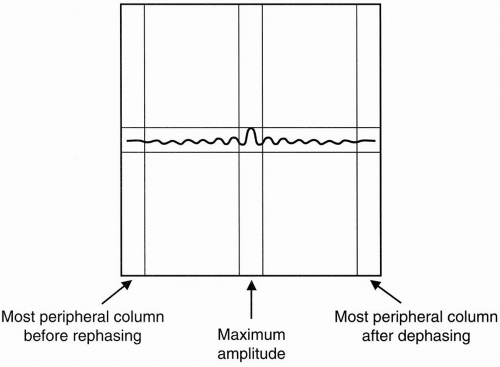Figure 13-3. The peripheral points in the signal have the weakest amplitude; the center point has the maximal amplitude.

As we go farther out to the periphery in both directions, the signal weakens:

In the y direction because of progressively larger phase-encoding steps
In the x direction because the echo signal has either not yet reached maximum amplitude or is losing maximum amplitude due to dephasing

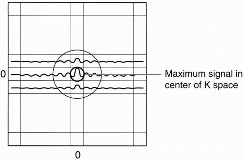Figure 13-4. The center of k-space always contains maximum signal.

Image of k-Space. Because of the oscillating nature of the signals, the image of the data space (and, thus, k-space) will appear as a series of concentric rings of signal intensity with alternating bands of high and low intensity as the signal oscillates from maximum to minimum, but an
overall decrease in intensity as one goes from the center to periphery (Fig. 13-5A). So, the white and dark rings in k-space correspond to the peaks and valleys of the echoes, respectively. The original raw data (k-space) and the original image are shown in Figure 13-5.

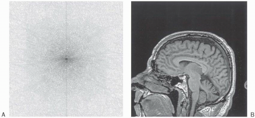Figure 13-5. A: The original raw data (k-space) of (B) the original image (midline sagittal T1-weighted image of the brain).

Edges of k-Space. You might be thinking that if the center of k-space contains the maximum signal, why not eliminate the periphery of the signal and just make an image from the central high signal intensity data (Figs. 13-4 and 13-6A)? We can actually make an image with this data, but the edges of the structures imaged will be very coarse (Fig. 13-6B). The periphery of k-space contributes to the fine detail of the image. Let’s see how this happens.

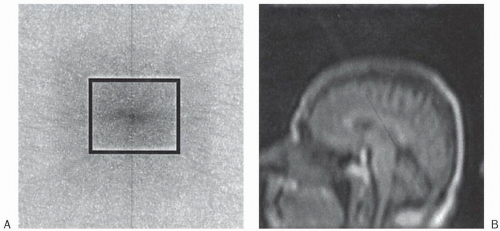Figure 13-6. A: k-Space. B: The image constructed from only the center of k-space. The details are reduced due to exclusion of peripheral points in k-space.

Question: What type of information is available in the periphery of k-space?

Answer: The periphery of k-space provides information regarding “fineness” of the image and clarity at sharp interfaces.

Recall the following Fourier transforms of a sinc wave and its truncated version from an earlier chapter (Fig. 13-7). As you can see, by truncating
the signal (echo), ring artifacts are introduced in the Fourier transform. Therefore, by eliminating the samples in the periphery of the data space, the sharp interfaces in the image are degraded and the image gets coarser. In other words, the fine detail of the image is compromised when the edges of k-space are excluded. Figure 13-8B is the image corresponding to the periphery of k-space (Fig. 13-8A).

Figure 13-7. A: The FT of an ideal sinc function is a rectangle. B: The FT of a truncated sinc function has ring down effects.

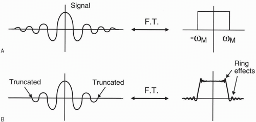Image Construction. We can take a single line in k-space and make a whole image. It wouldn’t be a very pretty image, but it would still contain all the information necessary to construct an image of the slice.

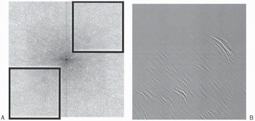Figure 13-8. A: k-Space. B: The image constructed from only the periphery of k-space. This image has minimal signal but contains details about the interfaces in the original image.

There is absolutely no direct relationship between the center of k-space and the center of the image. Likewise, there is no direct relationship between the edges of k-space and the edges of the image.

A point at the very edge of k-space contributes to the entire image. It doesn’t contribute as much to the image in terms of the SNR as does a point
in the center of k-space because the center of k-space has maximum signal, but the peripheral points still contribute to the clarity and fineness of the image.

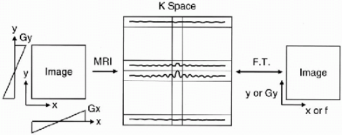Figure 13-9. There is a one-to-one relationship between frequency and position along the x-axis and between phase-encoding gradient increment and position along the y direction.

Once we have all the data in k-space, we take the Fourier transform of k-space to get the image.

Question 1: Why is the Fourier transform of k-space the desired image?

Answer: Because there is a one-to-one relationship between frequency and position in the x direction and between phase-encoding gradient strength¹ and position in the y direction.

Question 2: Why is there a one-to-one relationship between frequency and position?

Answer: Because, in our method of spatial encoding, we picked a linear gradient in the x direction that correlated sequential frequency increments with position; likewise, we picked a linear gradient in the y direction that correlated sequential phase gradient increments with position in the y direction (Fig. 13-9).

Thus, the center of the field of view of the image experiences no frequency gradient and no phase gradient, and the points in the periphery of the image experience the highest frequency and phase gradients. In other words, there is a 1:1 relationship between frequency and position in the image.

In summary, the frequency- and phaseencoding gradients provide the position of a signal in space. They tell us which pixels each component of the signal goes into in the slice under study.

Question: How are the shades of gray determined?

Answer: The shades of gray are determined by the magnitude

Only gold members can continue reading. Log In or Register to continue