(1)
where
 is the estimated source strength in nAm for a source at a given target voxel, and with a certain orientation; B is a vector containing the recorded magnetic flux at a given latency.
These weights are optimal in the sense that the values of the weights are chosen such that activity would be fully reconstructed for a target location, if this target location happens to be active (this is called the unit-gain constraint), whilst rejecting the contribution from all other sources, be it within or outside the brain. For a mathematical description we refer the reader to Robinson and Vrba 1999; Sekihara and Nagarajan 2008; van Veen et al. 1997, and for a review see Hillebrand et al. 2005).
Although other source reconstruction approaches also require accurate MEG/MRI co-registration and modeling of the volume conductor, beamforming is particularly sensitive to inaccuracies in the forward solution (Hillebrand and Barnes 2011, 2003; Vrba 2002): the unit-gain constraint described above results in a suppression of source activity if there is a deviation from the correct forward solution.
Equation 1 assumes that the orientation of a source is known. In practice, this is not the case, and the orientation can be set to the one that gives the maximum beamformer output (scalar beamformer; Robinson and Vrba 1999; Sekihara et al. 2004), the orientation of the cortical surface could be used (but see Hillebrand and Barnes 2003), or one could estimate the beamformer output for three orthogonal directions (vector beamformer; van Veen et al. 1997). Finally, the decrease in sensitivity for deeper sources (Hillebrand and Barnes 2002) results in an increase in the (norm of) the beamformer weights with source depth, and a disproportionate amplification of white sensor noise for deeper sources. To compensate for this depth bias, the beamformer weights, or equivalently the reconstructed beamformer image (Cheyne et al. 2006), are typically rescaled using a (projection of) the sensor noise. An estimate of the sensor noise therefore has to be provided. The effects of noise can further be reduced through regularization (Vrba 2002).
Once the beamformer weights have been estimated, one can reconstruct a three-dimensional volumetric image of activity (or of a change in activity in case experimental conditions are contrasted; see also Brookes et al. 2005). The statistical significance of these individual images is difficult to determine (but see Barnes and Hillebrand 2003), yet one can readily perform group-level statistics using tools developed for functional Magnetic Resonance Imaging (fMRI; Singh et al. 2002, 2003). We have recently introduced an atlas-based approach that also enables the comparison of beamformer results across individuals (see Fig. 1; Hillebrand et al. 2012). For each individual, the neuronal activity is reconstructed for a limited set of regions-of-interest (ROIs) that covers almost the entire brain, where the ROIs can be obtained from a standard atlas (Collins et al. 1995; Evans et al. 2012; Lancaster et al. 1997, 2000; Tzourio-Mazoyer et al., 2002). This approach has two main advantages: i) it enables the comparison between different modalities (Bullmore and Sporns 2009); ii) the number of ROIs is always the same across individuals, such that functional networks can more readily be compared (but see below).
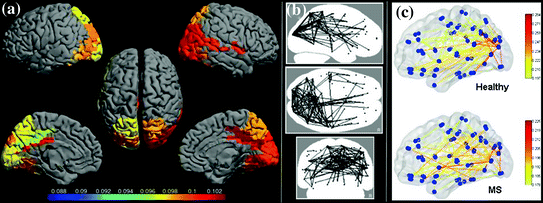

Fig. 1
Examples of recent applications of an atlas-based beamformer in combination with functional network analysis. Panel a shows data from a group of 13 healthy controls. The mean alpha band PLI, also known as the weighted degree or node strength in terms of graph theory, for each ROI, is displayed as a color-coded map (thresholded at p = 0.05) on a schematic of the parcellated template brain (modified from Hillebrand et al. 2012). Note that the regions in the occipital lobe are most strongly connected, as can be expected for the alpha band. Panel b shows the connections (PLI) from each ROI to all other ROIs, using an arbitrary threshold. Again, there is a clear pattern of strong connections between regions in the occipital lobe, with additional connections to areas in the temporal and frontal lobes. The upper panel in c shows a similar patterns for data from 17 healthy controls from a different study (Tewarie et al. 2014). This figure displays only the connections that formed part of the MST in the alpha2 band (the colorbar indicates PLI values). Interestingly, there seems to be a shift from an occipital to frontal pattern in healthy controls to a more diffuse pattern in 21 patients with Multiple Sclerosis (lower panel) (modified from Tewarie et al. 2014). Moreover, Tewarie and colleagues showed that this change in network topology correlated with reduced overall cognitive performance
3 Functional Connectivity in Source-Space
The recorded MEG data can be projected through the estimated beamformer weights in order to obtain the time-series for each voxel in the brain (Eq. 1), which are often referred to as virtual electrodes. In order to obtain a single time-series for each ROI, we subsequently select the voxel with maximum power as representative for the ROI. These ROI time-series can then be used as input for functional connectivity analysis. A wide range of functional connectivity estimators are available (Pereda et al. 2005), yet most of these measures are sensitive to the effects of volume conduction and field spread. One could remove these biases before performing connectivity analysis (Brookes et al. 2012; Hipp et al. 2012), or estimate the extent of the bias through simulations (Brookes et al. 2011a). Perhaps more straightforward is the use of measures such as the imaginary part of coherency (Nolte et al. 2004), phase-slope index (Nolte et al. 2008), the Phase Lag Index (PLI; Stam et al. 2007) and related lagged phase synchronization (Pascual-Marqui 2007), as these are inherently insensitive to these biases, where the PLI has the additional advantage that it does not directly depend on the amplitude of the signals (but see Muthukumaraswamy and Singh 2011). These measures have therefore gained popularity in recent years (Canuet et al. 2011, 2012; Guggisberg et al. 2008; Ioannides et al. 2012; Martino et al. 2011; Nolte and Muller 2010; Ponsen et al. 2013; Sekihara et al. 2011; Shahbazi et al. 2012; Tarapore et al. 2012).
The PLI is defined as (Stam et al. 2007):
![$${\text{PLI }} = \left| {\left\langle {{\text{sign}}\left[ {\sin \left( {\Delta \phi ({\text{t}}_{\text{k}} )} \right)} \right]} \right\rangle } \right|,$$](/wp-content/uploads/2016/04/A272390_1_En_12_Chapter_Equ2.gif)
where Δϕ is the difference between the instantaneous phases for two time-series defined in the interval [−π, π], tk are discrete time-steps, and < > denotes the mean. In short, PLI is a measure for the asymmetry of the distribution of phase differences between two signals, and ranges between 0 and 1. A PLI value of 0 indicates no coupling, coupling with a phase difference of 0 ± nπ radians (with n an integer), or an equal distribution of positive and negative phase differences. Common sources lead to a phase difference of 0 ± nπ radians between two signals, hence the PLI is insensitive to the influence of common sources (Stam et al. 2007). A PLI > 0 is obtained when the distribution of phase differences is asymmetric and is indicative of functional coupling between two signals. Note that PLI does not indicate which of the signals is leading in phase (but see Stam and van Straaten 2012a) and that it potentially discards true interactions with zero-phase lag. Moreover, a value of 0 for uncoupled sources is only achieved for (infinitely) long time-series, hence the PLI is affected by the length of the time-series. PLI also underestimates connectivity between sources with small-lag interactions. A modification of PLI addresses this issue, albeit at the expense of introducing an arbitrary bias favoring large phase differences and mixing of the estimation of consistency of phase differences with the estimation of the magnitude of the phase difference (Vinck et al. 2011).
![$${\text{PLI }} = \left| {\left\langle {{\text{sign}}\left[ {\sin \left( {\Delta \phi ({\text{t}}_{\text{k}} )} \right)} \right]} \right\rangle } \right|,$$](/wp-content/uploads/2016/04/A272390_1_En_12_Chapter_Equ2.gif)
(2)
4 Topology of the Functional Network
Graph theory provides the mathematical framework to characterize the topology of the functional network that is formed by the interacting sources. For this purpose, each ROI is denoted as a vertex (node) and each connection (e.g. the PLI value) is denoted as an edge between the vertices (see Fig. 1). Various graph-theoretical measures can subsequently be used to characterize the network (e.g. Rubinov and Sporns 2010). Two such measures, the clustering coefficient2 and the (average shortest) path length,3 can be used to explain how the brain can fulfill two seemingly contradictory requirements, namely the processing of information in local functional units on the one hand (‘segregation’) and simultaneous coordination of activity in and between these spatially separated units (‘integration’) (Sporns et al. 2002, 2004). Watts and Strogatz (1998) famously demonstrated with a simple rewiring model that adding a few long distance connections to a network with many local interconnections results in a high clustering yet small average path length. Many large networks, including the brain, have such a so-called small-world configuration (Bassett and Bullmore 2006; Stam 2004). However, this model does not provide a completely satisfactory description of functional brain networks, since it can not explain the occurrence of hubs (Eguiluz et al. 2005). Similarly, the scale-free growth model by Barabasi and Albert (1999), which explains the occurrence of hubs, does not capture the high level of clustering and (hierarchical) modularity observed in experimental data (Meunier et al. 2009). Obviously, we currently lack a model that integrates small-world and scale-free models and fully and elegantly explains the observed functional brain network characteristics (Bullmore and Bassett 2011; Clune et al. 2013; Stam and van Straaten 2012b).
From a practical point of view, although the application of graph theory at the source-level already aids the interpretation of results and the comparability across studies, it is not trivial to compare network topology across individuals, groups, studies or modalities, as was elegantly shown by van Wijk et al. (2010). At the heart of the problem lies the observation that many network properties depend on the size, sparsity (percentage of all possible edges that are present), and the average degree (i.e. the average number of connections per node) of the network. Fixing the number of nodes and average degree in the network (by setting a threshold) does eliminate size effects but may introduce spurious connections or ignore strong connections in the network, and using random surrogates for normalization does not solve this problem either (and may even exuberate it; van Wijk et al. 2010).
A novel approach is to construct the minimum spanning tree (MST) of the original graphs (Boersma et al. 2013; Jackson and Read 2010a, b; Wang et al. 2008). A tree is a sub-graph that does not contain circles or loops and connects all nodes in the original graph, and the MST is the tree that has the minimum total weight (i.e. the sum of all edge values4) of all possible spanning trees of the original graph. If the original graph contains N nodes than the MST always has N nodes and M = N−1 edges, therefore enabling direct comparison of MSTs between groups and avoiding aforementioned methodological difficulties. Furthermore, if the original network can be interpreted as a kind of transport network, and if edge weights in the original graph possess strong fluctuations, also called the strong disorder limit, then all transport in the original graph flows over the MST (van Mieghem and van Langen 2005), forming the critical backbone of the original graph (van Mieghem and Magdalena 2005; Wang et al. 2008). Interestingly, it seems that for source-reconstructed MEG data for patients with Multiple Sclerosis, as well as for healthy controls, there is a tendency of the weight distribution towards the strong disorder limit (Tewarie et al. 2014). This implies that there is a high probability that the MSTs for both patients and healthy controls can be considered as the critical backbone of the original functional brain networks. Hence, analysis of the minimum spanning tree not only provides a bias free approach to network analysis, but also captures important properties of the original network.
5 Applications in Neurology
5.1 Glioma
In a recent MEG study we revealed a relationship between resting-state functional network properties and protein expression patterns in tumor tissue collected during neurosurgery (Douw et al. 2013). In particular, between-module connectivity was selectively associated with two epilepsy-related proteins, namely synaptic vesicle protein 2A (SV2A) and poly-glycoprotein (P-gp), yet only for the ROIs that contained tumor tissue. Moreover, receiver operator characteristic (ROC) analysis revealed that SV2A expression could be classified with 100 % accuracy on the basis of the between-module connectivity, indicating that the role of the tumor area in the brain network may be an excellent marker for molecular features of brain tissue, which may be used clinically to monitor the efficacy of the anti-epileptic drug levetiracetam (de Groot et al. 2011


Stay updated, free articles. Join our Telegram channel

Full access? Get Clinical Tree


