Chapter Outline
Principles of Diffusion-Weighted Imaging
Clinical Application in the Abdomen
Diffusion-weighted magnetic resonance imaging (MRI) was introduced into clinical practice in the mid-1990s, primarily in brain imaging because of its exquisite sensitivity to detect ischemic infarcts. In the past decade, technical advancements have allowed the technique to be translated to body imaging, and abdominal diffusion-weighted imaging (DWI) is now well established. The clinical applications of abdominal DWI are both oncologic and nononcologic; the oncologic applications have been especially helpful.
DWI provides a contrast mechanism for the qualitative and quantitative assessment of tissues. The technique is complementary to and in some situations a viable alternative to gadolinium-enhanced MRI. Abdominal DWI does not require contrast media to be administered, yet it frequently highlights pathologic processes visible on contrast-enhanced techniques with increased conspicuity. The technique allows disease detection and assessment beyond that achievable by morphologic imaging alone.
This chapter discusses the principles of DWI, technical implementation, image interpretation, clinical applications, and potential pitfalls of the technique as applied to imaging of the abdomen.
Principles of Diffusion-Weighted Imaging
At its most fundamental level, DWI uses an imaging sequence that probes the microscopic mobility of water. The true diffusion coefficient of water is a measure of the effective displacement of water molecules per unit time, which is a random process (brownian motion) and is temperature dependent. Conceptually, it may be useful to consider the diffusion coefficient as a reflection of the freedom of movement of water molecules in a particular volume.
Several biophysical mechanisms can alter the random brownian motion of water molecules in tissues. These include cellular density, cell membrane integrity, cellular structural organization, and the presence of macromolecules that bind to water. The term apparent diffusion coefficient (ADC) represents the observed diffusion constant as the water molecules in tissues are modified by these biophysical interactions.
The image contrast on diffusion-weighted images is based on the differences in the diffusivity of water molecules. For example, tumor tissues exhibit low water diffusivity (or “impeded diffusion”) because of the relatively high density of cellular membranes. This increases the frequency of water proton–cell membrane interactions, which thus impedes water mobility. By contrast, a simple cyst containing water only would show high diffusivity as there are no barriers to water diffusion ( Fig. 69-1 ).

Observing and Measuring Water Diffusion with Magnetic Resonance Imaging
The quantification of diffusion with MRI on current clinical systems is based on experiments by Stejskal and Tanner in the1960s. The introduction of a pair of symmetric gradients before and after the 180-degree refocusing pulse of a conventional T2-weighted spin-echo sequence “sensitizes” the sequence to water motion ( Fig. 69-2 ). Static water spins dephased by the first gradient lobe would experience a complete rephasing by the second gradient lobe, thereby maintaining their signal. However, moving water spins will be in a different position at the time of the second lobe and thus not be rephased by the same degree, resulting in signal attenuation. Thus the presence of water diffusion is observed as signal loss on DWI. The greater the displacement of water molecules (i.e., the higher their diffusivity), the greater will be the degree of signal attenuation.

As with any MR sequence, the image contrast on DWI results from a combination of different tissue magnetic properties. In DWI, as this is significantly affected by water diffusion, the term diffusion weighted is used. However, the image contrast is influenced by both the underlying sequence (usually a T2-weighted sequence with a relatively long repetition time) and the strength of the diffusion weighting, which is given by the b value (diffusion weighting factor). The b value on a clinical scanner is usually altered by changing the amplitude of the diffusion sensitizing gradient, although it may be possible to vary the gradient duration and time interval between the paired gradients.
A b factor of zero (b = 0 s/mm 2 ) indicates no diffusion weighting, and the image is analogous to a T2-weighted image. In the abdomen, lower b values applied often range from 50 to 150 s/mm 2 ; higher b values typically range between 500 and 1000 s/mm 2 . DWI in the abdomen is usually performed with use of at least two b values, a lower and a higher b value. To calculate the quantitative ADC value, the relative signals of each voxel at different b value are mathematically fitted by an exponential function according to the following equation:
ADC = ln ( S 1 /S 0 ) / ( b 1 − b 0 )

Intravoxel Incoherent Motion Model
In certain organs such as the liver, the measured signal declines sharply with increasing diffusion weighting over the lower range of b values (typically 0-100 s/mm 2 ); the signal then attenuates more gradually with further increase in the b values. This biexponential behavior of signal attenuation is attributed to intravoxel incoherent motion (IVIM), in which intravascular microcapillary perfusion generates a pseudodiffusion effect at low b values. Thus, in calculating ADC values, the inclusion of these low b values can result in overestimation of tissue diffusivity. At higher b values, the pseudodiffusion effect is largely negated, and estimation of tissue diffusivity in tissues with significant tissue perfusion may be more reliable if the lower b values are excluded. However, the more sophisticated approach is to apply the biexponential IVIM model to the data fitting, from which the pseudodiffusion coefficient (D*), perfusion fraction (f), and tissue diffusion coefficient (D) are derived ( Fig. 69-4 ). Both D* and f reflect tissue perfusion and can vary independently.

The contribution of microcapillary perfusion may be considered in quantitative DWI analysis and is more significant in certain organs and pathologic processes. However, the utility of IVIM-based quantitative metrics is still largely confined to research, as accurate estimation of the perfusion-sensitive parameters can be challenging, particularly in lesions with inherently low vascular perfusion. Furthermore, there is currently a lack of commercial software for data analysis. Nonetheless, emerging observations suggest that in well-conducted studies with sufficient image signal-to-noise ratio (SNR) and in diseases or organs with significant perfusion effects, IVIM analysis may provide additional information to aid disease characterization.
Technical Considerations
Image Acquisition and Sequence Optimization
DWI sequences for clinical imaging of the abdomen are available on most current 1.5T and 3.0T MRI scanners. As in any MR sequence, tradeoffs between image spatial resolution, image SNR, and scan duration are often made, depending on the clinical indication. The technique that is most widely applied is single-shot fat-suppressed spin-echo echo planar imaging (SS-EPI). The primary merit of this technique is the speed of acquisition (with subsecond acquisitions of the entire k-space), but the sequence is prone to low SNR as well as ghosting, image distortion, blurring, and susceptibility artifacts. Other k-space acquisition techniques, such as multishot EPI DWI, turbo spin-echo DWI, and radial schemes of k-space acquisition (PROPELLAR DWI), may have potential to reduce some of the artifacts associated with the SS-EPI technique but are not widely implemented.
The underlying principles that guide imaging parameter selection in SS-EPI should be optimized for good SNR and reduction of artifacts. It is beyond the scope of this chapter to discuss the broader MR principles that affect image SNR and artifacts, but a few points that are particularly relevant to EPI DWI are mentioned here. First, fat suppression is routinely used to reduce the large chemical shifts in EPI and to increase the dynamic range of DWI images. This can be achieved either by inversion recovery (e.g., short tau inversion recovery) technique, which gives more uniform fat suppression but less SNR, or with chemical fat-selective saturation (e.g., spectral selected attenuation with inversion recovery or chemical shift selective imaging), which yields better SNR but is more susceptible to magnetic field inhomogeneities. Second, the echo time should be minimized as this increases the SNR; the repetition time should be sufficiently long to avoid T1 saturation effects (at least three to five times that of the T1 relaxation time of the imaged tissue). Use of a simultaneous gradient scheme (e.g., tetrahedral encoding or three-scan trace) allows the echo time to be reduced. Third, the number of signal averages can be increased to achieve better SNR, although at a cost of increased scan time. Some scanners allow the number of averages performed to vary with the b value, with more averages performed for SNR-poor high–b value DWI images. Last, parallel imaging should always be applied for body DWI as it shortens the echo train lengths, thereby reducing susceptibility and field inhomogeneity-related artifacts as well as reducing the acquisition time ( Tables 69-1 and 69-2 ). The reader is referred to the review article by Koh and associates for a more detailed discussion of the technical parameters that influence the imaging quality of EPI DWI images.
| Problem | Solution |
|---|---|
| Poor signal-to-noise ratio |
|
| Poor fat suppression and chemical shift artifact |
|
| Eddy current artifacts (geometric distortion, image shearing) |
|
| Nyquist (N/2) ghosting | Decrease receiver bandwidth |
| Parameter | Value |
|---|---|
| Pulse sequence | Single-shot spin-echo echo planar imaging |
| Imaging plane | Axial |
| Field of view, mm | 380 × 380 |
| Matrix size | 150 × 256 |
| Repetition time (TR), ms | 14,000 |
| Echo time (TE), ms | 72 |
| Echo planar imaging factor | 150 |
| Parallel imaging factor | 2 |
| Number of signals averaged | 4 |
| Section thickness, mm | 5 |
| Direction of motion-probing gradients | 3-scan trace |
| Receiver bandwidth | 1800 Hz/pixel |
| Fat suppression | Short tau inversion recovery (inversion time, 180 ms) |
| b value, s/mm 2 | 0, 100, 900 |
| Breathing technique | Free breathing |
| Acquisition time | 4 minutes 30 seconds |
Compensation for Physiologic Motion
Unlike in the brain, which is a reasonably static organ, several physiologic processes create motion-related phase artifacts in the abdomen that degrade image quality. This includes coherent movement, such as respiratory motion and bowel peristalsis, and noncoherent motion, such as cardiac pulsation.
Strategies to overcome artifacts arising from respiratory motion include breath-hold DWI, respiratory or navigator triggered/controlled DWI, and free-breathing DWI with multiple signal averages. Of these three techniques, breath-hold SS-EPI DWI of the abdomen is the fastest to perform, with coverage of the entire liver or abdomen over two breath-holds, each lasting approximately 20 seconds. The images retain good anatomic detail and are not degraded by respiratory averaging. However the major drawback is the lower SNR of the source data, which imposes limits on the acceptable spatial resolution (typically wider section thicknesses of 8 to 10 mm) and the maximum b value used (as higher b factors decrease the SNR). Fewer b values are obtained with this technique because of the limited number of b-value acquisitions that can be accommodated within a breath-hold. Breath-holding techniques may also be more sensitive to susceptibility and pulsation artifacts.
Respiratory or navigator triggered/controlled techniques synchronize data acquisition with respiratory movement, and data are acquired only within a certain period of the respiratory cycle (usually the expiratory phase). The advantages of this method include better subjective image quality, higher SNR, higher lesion-to-liver contrast ratio, and more precise ADC quantification compared with breath-hold DWI. However acquisition times are increased substantially (up to 5 to 6 minutes), and ADC measurements may be less reproducible compared with breath-hold and free-breathing DWI. In addition, the technique may result in pseudo-anisotropy artifacts related to the gated image acquisition.
In free-breathing EPI DWI, signal averaging from multiple acquisitions of the same imaging volume produces images with high SNR. Thin slice partitions (4-5 mm) are possible, and this allows multiplanar reconstructions of reasonable quality. A larger number of b values can be accommodated, which enables evaluation of ADC as well as IVIM parameters of lesions. However, image acquisition time is longer compared with breath-hold imaging (in the region of 3 to 6 minutes to cover the liver), and signal/volume averaging may result in suboptimal characterization of lesion heterogeneity, especially for smaller lesions. Even allowing for the presence of motion, ADC measurements in free-breathing DWI have been shown to be robust and comparable or even superior to breath-hold DWI.
Cardiac pulsation results in spin dephasing, which is most prominent in the structures immediately inferior to the heart, such as the left lobe of the liver, resulting in severe signal loss and overestimation of ADC. Cardiac gating seems intuitive to reduce cardiac motion effects in the liver, but some authors have found it difficult to find a phase of the cardiac cycle that yields diffusion-weighted images free of signal dropout artifact. Moreover, the combination of respiratory and cardiac gating will significantly prolong scan time to clinically unfeasible levels. Low–b value images are less prone to cardiac motion–induced signal loss and are therefore invaluable for lesion detection in susceptible areas.
Bulk motion from bowel peristalsis can be reduced by administration of antiperistaltic drugs (e.g., hyoscine butylbromide and glucagon). However, these are not routinely administered for the evaluation of the upper abdominal viscera.
Choice of b Values
There is no clear consensus on the precise number and magnitude of b values that should be used for abdominal DWI. Considerations include the target organ being evaluated, the image SNR, and whether DWI is primarily used for qualitative or quantitative analysis. For ADC quantification, three or more b values are generally recommended, with one being a lower b factor (≤100 s/mm 2 ) and one being a higher b factor (>500 s/mm 2 ). Additional b values can be considered to increase the accuracy of ADC estimation or if IVIM parameters need to be extracted with biexponential modeling. Increasing the number of b values results in increase in the imaging time. Some researchers now favor omitting b = 0 s/mm 2 in their ADC calculations to obtain perfusion-insensitive values for comparison between serial measurements.
Related posts:

Stay updated, free articles. Join our Telegram channel

Full access? Get Clinical Tree


