![]() To describe the Doppler effect and its application to the measurement of flow velocity.
To describe the Doppler effect and its application to the measurement of flow velocity.
![]() To understand the differences between continuous-wave and pulsed-wave Doppler and the clinical rationale for each.
To understand the differences between continuous-wave and pulsed-wave Doppler and the clinical rationale for each.
![]() To identify the components of the Doppler spectral waveform.
To identify the components of the Doppler spectral waveform.
![]() To recognize the aliasing artifact and understand the methods of reducing or eliminating it.
To recognize the aliasing artifact and understand the methods of reducing or eliminating it.
![]() To understand the principles of the two major types of color Doppler imaging.
To understand the principles of the two major types of color Doppler imaging.
KEY TERMS
Aliasing
Beat frequency
Color flow imaging
Color map
Color velocity scale
Color wall filter
Combined Doppler mode
Cutoff frequency
Doppler angle
Doppler effect
Doppler shift frequency
Doppler spectral waveform
Maximum velocity waveform
Packet size (ensemble length)
Power Doppler imaging
Spectral analysis
Velocity scale
INTRODUCTION
The ability to identify flow patterns and measure flow velocities is one of the most important functions of diagnostic ultrasound. The sonographer must understand the factors that contribute to the Doppler information displayed on the monitor. Most of what we discuss in this chapter applies to both spectral Doppler and color flow imaging, since and each mode is governed by the Doppler equation and is ultimately subject to the same factors.
THE DOPPLER EFFECT
The Doppler effect is the observed change in frequency of a transmitted wave due to the relative motion between the source of the sound and the receiver or observer. Doppler ultrasound is a valuable tool because this methodology detects the presence, direction, velocity, and time variation of blood flow within blood vessels and in the heart. Several types of Doppler devices are available. Although each relies on the Doppler effect to detect motion, the manner in which flow information is acquired, processed, and displayed distinguishes one type of instrument from another. Some scanners offer several Doppler modes, which are selectable by the user. The most basic (inexpensive) systems offer only a single option for the Doppler mode (velocity analysis or two-dimension Doppler imaging, i.e. color flow).
The apparent frequency change produced by the Doppler effect is based on the relative motion between the source of sound and the observer, regardless of which is moving and which is stationary. When a police car with siren blaring passes a pedestrian, the audible sound is heard as a change in frequency or pitch as the vehicle approaches (the frequency appears to be higher) while the frequency of the retreating vehicle after it passes is observed to be lower. In the above illustration, the sound source is the moving vehicle, while the receiver or observer is the stationary pedestrian.
Imagine a situation in which an observer is standing in a boat in the middle of a lake. If the wind is blowing at a constant rate from the north and the waves all have the same distance between peaks (same wavelength), the stationary boat will encounter the same number of wave crests each second (constant frequency) as are produced by the wind. If the boat begins traveling in a northerly direction, into the wind, the wave crests are encountered more frequently. The observer standing in the boat sees an increase in the wave frequency, although, in actuality, the frequency of the cresting waves has not changed. If the boat turns around and begins heading south, this time with the wind (away from the source of the waves), fewer crests are seen, and to the observer the frequency appears to decrease. As the boat moves faster in either direction, the difference between the actual and observed frequencies becomes greater. The only circumstance in which these “transmitted” and “observed” frequencies are the same is when the boat is stationary.
A stationary observer views the same number of pressure waves as are emitted by the stationary source (Figure 5-1). However, the relative motion between the sound source and the receiver distorts the pattern of symmetric wavefronts and the observed frequency increases or decreases, depending upon the direction of movement. The change or difference in frequency between the transmitted frequency and the received frequency, caused by the motion, is the Doppler shift frequency (often abbreviated as “Doppler shift” or “Doppler frequency”). In the example of the police siren above, the frequency appears higher to the stationary observer as the car approaches. In this case, the relative motion of the source and the receiver is toward one another. As the police car passes and travels away from the observer, the frequency appears to decrease, since the relative movement between the source and the observer is away from one another.
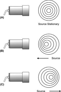
FIGURE 5-1. The Doppler effect. (A) Stationary sound source and receiver, the observed frequency is the same as the frequency emitted by the sound source. (B) Sound source moving toward the receiver, the observed frequency is higher than the actual frequency emitted by the sound source. (C) Sound source moving away from the receiver, the observed frequency is lower than the actual frequency emitted by the sound source.
When considering a sound wave produced by a piezoelectric transducer, the sound source remains stationary while the moving “receiver” could be blood cells or another moving structure, such as a heart valve. The echo from the moving reflector is then observed with a Doppler shift frequency by the stationary transducer, which is now the receiver.
Doppler Shift Equation
The magnitude of the Doppler shift frequency depends on how rapidly the sound source, the receiver, or both are moving in relation to one another. An increase in the relative velocity between the source and the receiver causes a greater deviation from the transmitted frequency. Indeed, this is the rationale behind why we perform the Doppler examination. The Doppler shift frequency (fD) produced by a moving reflector is calculated from the equation:

where c is the acoustic velocity of tissue, f is the transmitted frequency, v is the velocity of the interface, and θ is the angle between the path of reflector movement and the direction of beam propagation (called the Doppler angle or angle to flow) as illustrated in Figure 5-2. Note that the letter “c” in the Doppler equation represents the velocity of sound in tissue instead of the usual “v” for velocity. In this mathematical symbolism, the character “v” is reserved for the velocity of the flowing blood. The number 2 in the equation represents two separate (and equal) Doppler shifts that occur in Doppler ultrasound. The first Doppler shift occurs between the stationary sound source, the transducer, and the “observer,” the moving blood cells. The second Doppler shift takes place as the moving blood cells (now the sound source) reflect the sound wave back to the stationary transducer, which now becomes the receiver.

FIGURE 5-2. Doppler ultrasound detection of reflector velocity. The Doppler angle θ is defined by the reflector path with respect to the transmitted beam.
As a reflector moves directly toward a 5-MHz transducer at a velocity of 50 cm/s, the angle to flow is 0 degrees and the observed frequency is 5,003,247 Hz, corresponding to a Doppler shift frequency of 3247 Hz above the original transmitted frequency (Figure 5-3). If the flow is away from that transducer at 50 cm/s, the observed frequency is 4,996,753 Hz or 3247 Hz below the original transmitted frequency. The Doppler angle gives the component of the velocity along the direction of propagation for the ultrasound beam. If the Doppler angle is increased from 0 to 30 degrees, the Doppler shift frequency is 2.8 kHz instead of the 3.2 kHz obtained for parallel incidence. For a given reflector velocity, the Doppler shift frequency decreases as the Doppler angle is increased (Figure 5-4).
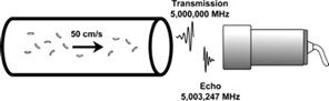
FIGURE 5-3. Received echo frequency is 3247 Hz above the transmitted frequency when the flow velocity is 50 cm/s toward the transducer. The transmitted frequency is 5 MHz and the Doppler angle θ is 0 degrees.
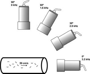
FIGURE 5-4. Doppler shift frequency from reflectors moving at a velocity of 50 cm/s versus Doppler angle. The transmit frequency is 5 MHz. The Doppler shift frequency is 3.2 kHz at 0 degrees, 2.8 Hz at 30 degrees, and 1.6 kHz at 60 degrees. No Doppler shift frequency is observed at 90 degrees.
No Doppler shift frequency occurs at a 90-degree angle of incidence (cosine theta in the Doppler equation is equal to zero for an incident angle of 90 degrees). In practice, the signal never disappears completely. Because the beam has a finite width, some portion of the beam impinges at an angle that is not perpendicular to the motion. Beam divergence tends to amplify this effect, especially in the region beyond the beam’s focal point.
Velocity Determination
The acoustic velocity is assumed to remain constant at a value of 1540 m/s for soft tissue. The observed change in frequency occurs because the sound beam encounters a moving structure between the source and the detector. The Doppler equation predicts that an increase in reflector velocity results in a greater Doppler shift frequency. If the Doppler shift frequency and angle to flow are known, the velocity of the moving reflectors can be calculated. In practice, the transmitted and received frequencies are first measured, and then processed to find the resultant Doppler shift frequency. The instrument accomplishes these steps autonomously without operator intervention. However, the Doppler angle to flow must be determined by the sonographer with manual input to the scanner for the correct display of flow velocity.
Uncertainty in the measurement of the Doppler angle, particularly at large angles, introduces error in the velocity computation. The exact angle to flow is much more of a consideration when evaluating blood vessels than in the heart due to differences in acoustic access. In vascular applications, the process of angle correction (angle measurement) must be performed by the sonographer in order to achieve an accurate estimation of flow velocity. At a Doppler angle to flow of 60 degrees, the resultant Doppler shift is only half that with a Doppler angle of 0 degrees. The angle to flow must be measured as accurately as possible, because a 5-degree deviation for a 60-degree angle to flow (frequently used when examining blood vessels) introduces an 18% error in the measurement of flow velocity.
Conversely, when the beam is near parallel to flow (as is frequently the case in the heart), the Doppler angle to flow is assumed to be 0 degrees and no angle correction is performed. At a Doppler angle to flow near 0 degrees, a 5-degree inaccuracy in the angle results in only a 1% error in the calculation of flow velocity. A 10-degree error in the estimation of Doppler angle to flow results in a velocity error of less than 10%. In practice, the angle of insonation is assumed to be 0 degrees in cardiac applications and no “angle correction” is performed.
Doppler signals from superficial blood vessels (e.g., the carotids) should generally not be acquired at angles greater than 60 degrees, due to the increased potential of error as the Doppler angle approaches 90 degrees. Regardless of the angle, care should be taken in vascular applications to measure the angle to flow as accurately as possible.
Scattering from Blood
For Doppler measurements of blood flow, red blood cells (RBCs) act as Rayleigh scatterers. The RBC has a diameter of 7 μ (much smaller than the wavelength of the sound wave, usually 0.2–0.5 mm) and thus meets the condition for Rayleigh scattering. Rayleigh scattering exhibits very strong frequency dependence (proportional to the fourth power of the frequency). Therefore, the intensity of the scattered ultrasound energy increases dramatically as the transmitted frequency increases.
The intensity of the scattered sound also depends on the number of RBCs and thus the quantity of blood in the sample volume. Because the scattering from blood is small compared with echoes produced by soft tissue interfaces, blood-filled vessels appear to be echo-free on the B-mode image. To enhance scattering and, therefore, increase the sensitivity to weak echoes generated from blood cells, a high-frequency transducer is often advantageous. However, at higher frequencies, the rate of attenuation of the sound beam by the intervening tissues becomes greater. Therefore, as with B-mode imaging, two opposing frequency-dependent effects (in the case of Doppler, penetration and scattered echo intensity) must be balanced by matching the transducer transmit frequency with the depth of the region of interest.
Doppler transducers usually operate in the frequency range of 2–10 MHz, because other constraints are placed on the system: a single transducer with dual imaging and Doppler functions, a desired frequency range for Doppler shift frequency, and the problem of aliasing (discussed later in this chapter). High transmit frequencies, typically 5–7 MHz, are employed for peripheral vascular Doppler examinations, whereas examinations of deep-seated vessels are performed at frequencies near 2 MHz. Most often, the transmitted Doppler frequency is somewhat lower than the nominal imaging frequency of the transducer. For example, a transducer labeled as “5 MHz” refers specifically to the B-mode imaging frequency. The transmitted frequency of sound used for Doppler evaluation in that same transducer will likely be in the range of 2–3 MHz. Some ultrasound instruments display the actual transmitted frequency used for Doppler, while others display only descriptors such as “resolution/penetration” while in the Doppler mode.
Doppler Display
Doppler units are designed to extract the Doppler shift frequencies from received signals. The Doppler shift frequency is in the audible range (typically between 200 and 15,000 Hz). Therefore, loudspeakers are used as output devices in addition to any other type of available display. Nearly all commercially available systems provide an audio display of the Doppler signal, as the human ear is extremely sensitive to Doppler signals. For visual display, the preferred format is to convert the measured Doppler shift frequency to velocity, which is independent of instrument parameters. Doppler displays utilizing frequency expressed in kilohertz, without velocity information, are not readily comparable when multiple examinations are performed by different sonographers on different instruments.
CONTINUOUS-WAVE DOPPLER
A continuous-wave (CW) Doppler transducer contains two piezoelectric elements: one to transmit the sound waves of constant frequency continuously and one to receive the echoes continuously (Figure 5-5). A single-element transducer cannot send and receive at the same time. Since the transmitted sound wave is not pulsed, broad bandwidth transducers are not practical or even appropriate (wide frequency range yields multiple Doppler shifts for a reflector moving at constant velocity).
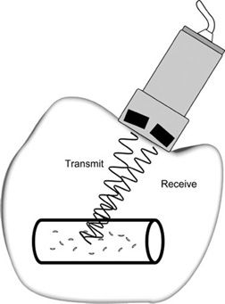
FIGURE 5-5. Continuous-wave Doppler transducer. Pencil-type probe has two piezoelectric crystals: one transmits continuously, the other receives continuously.
The sampling volume is restricted by the transmitted ultrasonic field (dependent on the frequency and focal properties of the sound beam) and the geometric arrangement of the elements. For the detection of a moving reflector located along the path of the transmitted beam, the resulting echo must strike the receiving crystal. The sensitive volume, or zone of sensitivity, is defined by the intersection of the transmitted ultrasound field and the reception zone. In essence then, each two-element transducer is focused to a particular depth (Figure 5-6). The two elements are tilted slightly to allow overlap between their respective fields of view (transmission and reception). A multiple-element array transducer creates a similar zone of sensitivity in CW Doppler mode by dedicating one group of elements as the transmitter and another group as the receiver (Figure 5-7).
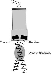
FIGURE 5-6. Zone of sensitivity for CW Doppler transducer.
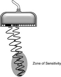
FIGURE 5-7. Multiple-element array transducer operating in CW Doppler mode. One group of elements (black) is designated for transmission and another group (gray) is assigned for reception. A zone of sensitivity is created where the wave patterns overlap.
Depending on the clinical application, the sonographer selects a CW transducer with the appropriate operating frequency and sensitive region. In a multiple-element array transducer, the operating frequency and depth of the sensitivity zone in CW Doppler mode may be adjustable, depending upon the instrument.
Doppler Measurement
The transmitted sound wave interacts with various reflectors, some of which are stationary and others moving. A fraction of the incident sound intensity is reflected at each interface. If the reflector is stationary, the frequency of the reflected sound wave is the same as the transmitted frequency, and consequently no change in frequency is observed. A moving interface causes the frequency of the echo to shift up or down depending on whether the movement is toward or away from the sound source.
Measurement of the Doppler shift frequency is based on the principle of wave interference. The Doppler effect causes the reflected wave received from a moving interface to vary slightly in frequency from the original transmitted wave. When waves with different frequencies are algebraically added together, they yield a slowly oscillating broad pattern of peaks and valleys, called the beat frequency (Figure 5-8). The beat frequency equals the difference in frequency between the two waves (transmitted and received) and thus corresponds to the Doppler shift frequency.
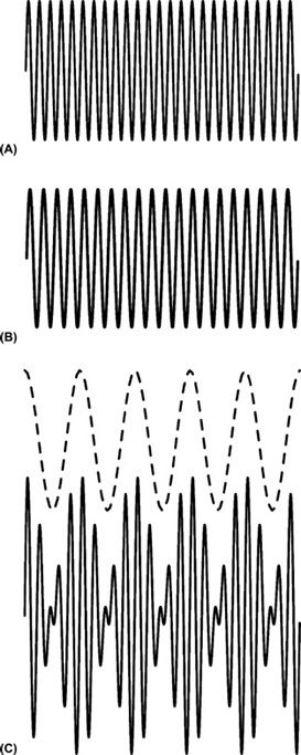
FIGURE 5-8. Doppler signal processing. (A) Continuous reference transmitted signal of constant frequency (25 cycles). (B) Continuous echo-induced signal of constant frequency (20 cycles). (C) Addition of the transmitted and received signals in A and B forms a complex waveform. The beat frequency of five cycles composes the outer envelope (dotted line) of this complex waveform.
Figure 5-9 illustrates the steps required to generate the Doppler signal. The oscillator regulates the transmitter to emit a continuous sound wave of a single frequency. Alternating pressure on the receiving element by the returning echo is converted to an RF (radiofrequency) signal. The amplifier increases the echo-induced signal level. The reference waveform from the oscillator, which mimics the transmitted wave, is then combined with the received signal at the demodulator, generating complex resultant wave by means of wave interference. This resultant wave is then processed to remove the rapidly oscillating components; however, the slowly varying envelope corresponding to the beat frequency (dotted line in Figure 5-8C) is retained. Isolation of the beat frequency yields the Doppler signal, which has a frequency equal to the Doppler shift frequency.
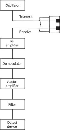
FIGURE 5-9. Schematic showing components of a continuous-wave Doppler unit.
Complex Doppler Signal
The signal processing illustrated by Figure 5-8 yielded a single-beat frequency, which denoted reflectors moving at a single, constant velocity. In a Doppler ultrasound examination of blood flow, RBCs within a vessel have a range of velocities that vary throughout the heart cycle and therefore, a range of Doppler shift frequencies will be present. The velocity of each moving reflector corresponds to a characteristic beat frequency upon echo detection and processing. Many beat frequencies representing all detected motion within the sampling volume comprise the Doppler signal. A complex Doppler signal is then formed by the summation of all the Doppler shift frequencies present after demodulation.
Signal Processing
The complex Doppler signal is amplified, filtered to remove unwanted low-frequency components caused by slow-moving structures such as vessel walls, and then routed to a loudspeaker for audible “display.” The pitch of the audio output corresponds to the frequency shift between the transmitted and received sound waves and indicates the flow velocity within the vessel. As flow velocity becomes greater, a higher pitch is heard. A typical audio Doppler display for an artery exhibits a rhythmic rise and fall in the audible frequency due to the acceleration and deceleration of blood with systole and diastole.
Large, slow-moving specular reflectors in the body (e.g., vessel walls or heart valves) generate strong echoes with relatively low Doppler shift frequencies. These low frequencies produce a distracting thumping sound often referred to as “wall thump.” Filtering removes these low frequencies, which are normally not of major interest and could mask other signals. The operator control, wall filter, rejects all frequencies below the threshold value, known as the cutoff frequency (Figure 5-10).
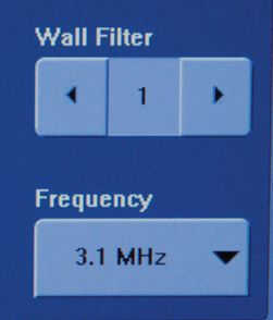
FIGURE 5-10. Wall filter control.
The cutoff frequency is usually set by default to remove Doppler shift frequencies below 100 Hz. Depending on the manufacturer and model, the cutoff frequency can be adjusted to values as low as 40 Hz and as high as 1000 Hz (1 kHz). Most units automatically set the threshold value based on the study type selected in the preset menu. Because the wall filter control removes all frequencies below the cutoff value, care must be taken so that slow-moving flow is not excluded from the display. Thus, the wall filter should be set at the lowest possible value to remove wall thump while not eliminating any important blood-flow components of the Doppler signal. This is particularly true for slow venous flow as well as for the slight flow reversal that occurs in a normal triphasic arterial waveform (discussed in the following chapter).
Clinical Aspects
CW Doppler has high sensitivity to detect slow flow with low Doppler shift frequencies and, further, can discriminate small differences in flow velocity (Figure 5-11). The long sampling time of CW Doppler enables this modality to identify small changes in frequency corresponding to slow flow. At the other extreme, high-velocity flow is accurately measured with no limitation in velocity range. However, extensive flow volumes, such as those encountered within the left ventricle, cannot be accurately assessed with CW Doppler because precise depth information is not possible. The observed Doppler signal can be extremely complex, because the sum of Doppler shifts generated by all the moving interfaces within the sensitive volume is portrayed. If the sampling volume includes multiple vessels, the superposition of resulting Doppler shifts becomes especially problematic. Therefore, CW Doppler is limited to those clinical applications in which sensitivity volume can be associated with a single vessel, such as the brachial or femoral artery. CW Doppler is commonly employed to evaluate flow patterns in heart valves. In this case, even though the large sampling area of CW Doppler records flow from other portions of the atria and ventricles, the easily recognizable flow pattern of the aortic and mitral valves is readily identified. Coupled with the fact that CW Doppler has essentially no practical limit to the velocity that can be measured, this modality is ideal to assess stenosis in valves, such as the aortic valve. (Aortic stenosis often produces velocities in the range of 500–600 cm/s, which would be impossible to determine accurately with a pulsed-wave (PW) Doppler system.)
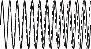
FIGURE 5-11. Sensitivity of continuous-wave Doppler to slow flow. The echo-induced signal from a slow-moving reflector (dotted line) requires several cycles to be differentiated from the reference transmitted signal (solid line).
PULSED-WAVE DOPPLER
PW Doppler provides quantitative depth information of the moving reflectors. Depth of echo formation is obtained via the echo-ranging principle in similar fashion to B-mode imaging. The transducer is electrically stimulated to produce a short burst of ultrasound and then is silent to listen for echoes before another pulsed wave is generated. Because of the requirement to assign depth, there is a physical limit to the number of Doppler pulses that can be transmitted in a given amount of time. Also, Doppler shift frequency determination entails longer pulse duration than in B-mode imaging. The necessity for increased pulse duration lies in the desire to detect received frequencies associated with slow flow that are almost the same as the transmitted frequency. Imagine that the pulse duration was confined to three cycles as in a typical B-mode acquisition (Figure 5-12). Certainly, the ability to distinguish small changes compared with the transmitted frequency becomes more difficult as pulse duration is shortened.
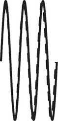
FIGURE 5-12. Pulsed-wave transmission of few cycles is unable to detect low-velocity reflector. Reference transmitted signal (solid line) and echo-induced signal (dotted line) are nearly identical.
The received signals are electronically gated for processing so only the echoes that are detected in a narrow time interval after transmission, corresponding to a specific depth, contribute to the Doppler signal. The delay time before the gate is turned on determines the depth of the sample volume; the amount of time the gate is activated establishes the axial length of the sample volume (Figure 5-13). Gate parameters are selected by the operator; thus, the axial size of the sensitive volume and the depth of the sample can be adjusted. The axial sample length can be as small as 1 mm. The remaining dimensions of the sampling volume are dictated by the beam width in the in-plane direction and in elevation direction. Figure 5-14 illustrates the designation of the sampling region along the Doppler scan line in a B-mode image. Transducer frequency and focusing characteristics influence the dimensions of the ultrasonic field.
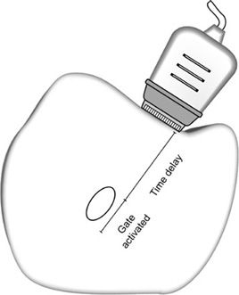
FIGURE 5-13. In pulsed-wave Doppler, the timing gate determines the depth and axial length of the sampling volume.
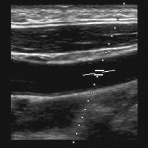
FIGURE 5-14. Operator-defined sampling area for pulsed-wave Doppler. The dotted line indicated the direction of sampling and parallel horizontal lines mark the axial extent of the sensitive region.
Multiple echoes from a moving reflector separated in time must be accrued to detect the motion. In order to achieve this, transmitted pulses are repeatedly directed along the same scan line to interrogate the sampling volume. Suppose a photographer took a single stop-action photograph (with an extremely short shutter time) of a car traveling west at 60 miles per hour. If you were shown that photograph, you would be unable to tell if the car was moving or not. And certainly, the direction of travel and speed would be indiscernible. However, if a series of stop-action photographs were acquired over a specific time period and then shown rapidly one after the other, the motion of the car would be clearly depicted, and the speed could be computed if the rate of sampling were known.
In PW Doppler, the basic CW design is modified to accommodate range gating and to collect successive processed echoes for analysis. Accurate time registration is critical for proper depth assignment of the Doppler signals. Gating is based on elapsed time following each transmitted pulse, and the time between consecutive echoes from a reflector is set by the pulse repetition period (PRP). The PRP is the time interval from the beginning of one transmit pulse to the beginning of the next transmit pulse. A single gate limits the interrogation to one depth along the scan line. The direction of sampling is indicated on the display by the Doppler cursor. Echoes formed along the Doppler scan line, but outside the sampling volume, are rejected. Only those echoes generated from within the sampled volume contribute to the Doppler display.
For reflectors moving at uniform and constant velocity within the sampling volume, a series of echoes from successive transmitted pulses are acquired over time. The depth-specific echo from each transmitted pulse, when processed, provides a single instantaneous value of the Doppler signal (beat frequency). The measured values obtained from multiple transmitted pulses are combined to form the time-varying contour of the Doppler shift frequency (Figure 5-15). In essence, the transmitted pulse rate (Doppler pulse repetition frequency or PRF) indicates how often the Doppler signal is sampled. Typically, a sequence of 64–128 pulses is transmitted along the line of sight to interrogate flow within the sample volume. The total observation time is usually 10 ms or less.
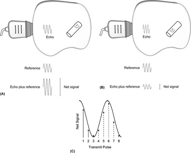
FIGURE 5-15. Pulsed-wave Doppler signal processing. A series of transmitted pulses are directed along the Doppler line of sight. (A and B) For each transmitted pulse, the echo-induced signal from moving reflectors within the sampling volume is combined with the reference signal to yield the net signal. The net signal from successive transmit pulses varies due reflector movement. Note the change in position of RBCs between transmit pulses in (A) and (B). (C) The net signals from multiple transmitted pulses when placed on a time axis compose the beat frequency. The first two points of sampling from A and B are shown as solid lines. Subsequent measurements are indicated by the dotted lines. Connecting all the data points yields the projected beat frequency.
In PW Doppler, the beat frequency is not as well defined as with CW Doppler, because the pulsed echoes are equivalent to sampling the Doppler signal at discrete intervals. The oscillatory pattern can be more accurately delineated if the sampling occurs repeatedly at short intervals. This requires a high Doppler PRF.
Blood flows with a range of velocities within the sample volume and gives rise to multiple Doppler shift frequencies. These combine via interference to yield a complex Doppler signal, which represents all flow velocities present in the sampled volume. Fortunately, methods have been developed to isolate the individual velocity components and then display this information in an easy to understand format.
Velocity Detection Limit
PW Doppler has a limit with respect to the maximum beat frequency that can be detected accurately. This upper frequency boundary is called the Nyquist limit, which is caused by discrete (noncontinuous) sampling. The maximum Doppler shift frequency equals one-half the sampling rate, given by the Doppler PRF. Noncontinuous sampling creates a very important impediment in PW Doppler. To accurately measure a fast moving reflector producing a high Doppler shift frequency, a rapid sampling rate is necessary; however, a high PRF restricts the depth that can be interrogated, because a specific time is required to receive the echoes arising from that depth before the next transmitted pulse. Thus, as the depth to the vessel or structure is increased, more time is required between transmit pulses, and the maximum Doppler shift frequency that can be measured becomes lower. The problem becomes more complex because the Doppler shift frequency is also proportional to the transmitted frequency. The most problematic situation for PW Doppler occurs for deep-lying structures with high-velocity flow in which the Doppler angle to flow is near 0 degrees. This combination of factors arises frequently in the Doppler evaluation of heart valves, particularly with disorders such as aortic stenosis in which the velocities can be very high.
Table 5-1 illustrates the effect of the depth of interest and transmitted frequency on the maximum velocity limit when angle to flow is unchanged. As the depth of interest is increased, the maximum reflector velocity that can be measured is decreased. Importantly, a low-frequency transducer allows higher velocities to be detected. A larger Doppler angle extends the maximum velocity limit. At a depth of 10 cm with 5 MHz transmitted frequency, the maximum velocity limit increases from 84 to 119 cm/s when the Doppler angle is changed from 45 to 60 degrees. This velocity constraint occurs because the motion of the reflector is sampled at discrete intervals and not continuously, as with CW Doppler ultrasound. In contrast with PW Doppler, CW Doppler has no maximum velocity limit. (Since the CW transducer is continuously transmitting, there is essentially no “pulse repetition frequency” and therefore no Nyquist limit).
TABLE 5-1 • Maximum Velocity Limit in Pulsed-Wave Doppler with Different Transmit Frequencies
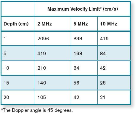
The following is a real-world example which illustrates a practical application of the maximum velocity limit in a Doppler examination. The maximum PRF for a 10 cm depth is approximately 7700 pulses per second. Using a 3.5-MHz transducer with a Doppler angle of 30 degrees, the maximum Doppler shift frequency, which can be accurately measured, is 3850 Hz, or a velocity of 98 cm/s. If the transmit frequency were lowered to 2 MHz, the maximum detectable velocity would increase to 171 cm/s. Changing the depth of interest to 15 cm while maintaining the transducer frequency at 3.5 MHz reduces the detectable maximum velocity to 65 cm/s. Fortunately, these conditions are such that the physiologic velocities of normal velocity blood flow (except within the heart) usually occur within the detectable range of PW Doppler units.
Aliasing
At a minimum, two measurements are required per beat cycle to define the Doppler shift frequency unambiguously. This is the reason the Nyquist limit (upper limit for detection of the Doppler shift frequency) is equal to one-half the Doppler PRF. Because the beat frequency is sampled intermittently in PW Doppler, limited data are available for calculation of the Doppler shift (each transmit pulse ultimately contributes one point on the waveform of the Doppler shift frequency). If the Doppler PRF is not adequate to generate at least two points per beat cycle of the Doppler shift frequency, the Doppler shift frequencies above the Nyquist limit will be misinterpreted as lower than their actual value (Figure 5-16). This error in the measurement of the Doppler shift frequency caused by a low sampling rate is called aliasing.
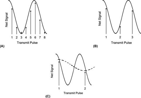
FIGURE 5-16. Intermittent sampling of the beat frequency (solid line). (A) Multiple measurements per cycle allow accurate assessment of the beat frequency. (B) As few as two measurements per cycle also provide accurate interpretation of the beat frequency. (C) If the sampling rate is less than two times per cycle, then the true beat frequency (solid line) is misinterpreted as a lower frequency (dotted line).
Imagine that a race car is traveling around an oval racetrack at constant speed. A series of photographs closely spaced in time would accurately depict the motion as the car advances around the track. Indeed, as long as at least two photographs are taken for each lap, the interpretation of the movement would be correct. Now suppose the car accelerates to a higher speed, while the frequency of the photographs remains unchanged. At this faster speed, there may be 1.5 photographs taken for each lap of the car (three photos every two laps). This series of photographs will now appear to show the car moving backward around the track at slower than the actual speed. Thus, there is a minimum sampling rate (2 photos per lap) that accurately portrays the motion of the car around the track, analogous to the minimum sampling rate, or PRF, in Doppler applications.
Because velocity information is almost always displayed in velocity units as opposed to frequency units, the Nyquist limit is typically given in velocity. The Nyquist limit may be displayed separately from the velocity scale; however, it is important for the sonographer to know that the Nyquist limit is equal to the maximum velocity shown on the scale. There are both a positive and a negative value displayed for the Nyquist limit. If the baseline is moved up or down from the middle of the spectral display, the maximum velocity limit for forward and reverse flow is no longer the same (Figure 5-17).
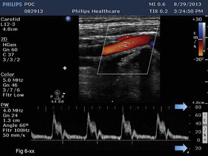
FIGURE 5-17. Baseline is placed off center. The maximum velocity in the forward and reverse directions is not the same (arrows). The + and – maximum velocity values are indicated by arrows.
If the baseline is moved all the way to the top or bottom of the spectral display, the Nyquist limit is extended to the greatest possible value in a single direction for the given sampling rate. However, any flow that is present in the opposite direction is unknown (Figure 5-18).
FIGURE 5-18. Baseline is moved to the bottom of the display. Measurements of velocity are restricted to one direction only, but the maximum velocity in the forward direction that can be displayed without aliasing is extended.
DUPLEX SCANNERS
Related posts:

Stay updated, free articles. Join our Telegram channel

Full access? Get Clinical Tree


