Fig. 9.1
PFC-in-water, PFC-in-oil-in-water and oil-in-PFC-in-water emulsions under the microscope
PFC liquids are known for their use in medicine due to their biocompatibility and inertness (Biro et al. 1987). PFC nanodroplet emulsions can be utilized for selective extravasation in tumor regions (Long et al. 1978). Due to their biocompatibility and suggested ability to passively target regions of cancer growth, PFC droplets represent an attractive tool for cancer diagnosis. PFC droplets may also extravasate and be retained in the extravascular space due to the enhanced permeability and retention effect in tumors (Rapoport et al. 2007; Zhang and Porter 2010). Extravasated droplets may be acoustically converted into gas bubbles allowing for ultrasound tumor imaging. At the same time PFC droplets are rich in fluorine, which makes them potential candidates as a contrast agent for MRI imaging. The availability of both intravascular contrast agents (microbubbles), and tumor-specific extravascular contrast agents (nanodroplets), would significantly increase diagnostic and therapeutic capabilities. Moreover, the droplets may be used to deliver chemotherapeutic agents to tumor regions, and locally release them upon exposure to triggered ultrasound (Rapoport et al. 2009).
9.2 Nonlinear Propagation
The amplitude of the acoustic pressure that is required to nucleate droplets in ADV turns out to be very high (Kripfgans et al. 2000). To obtain a sufficiently high pressure, a focused ultrasound transducer is applied and the droplet is placed in the focal area of the emitted beam. Moreover, the frequency of the emitted ultrasound wave is several MHz. In a typical ADV experiment, the ultrasound wave travels a few centimeters (Kripfgans et al. 2000; Reznik et al. 2013; Shpak et al. 2013a, b; Giesecke and Hynynen 2003; Schad and Hynynen 2010; Williams et al. 2013) before impinging on the droplet. The high pressure, high frequency, applied focusing and long propagation distances are all factors that strengthen the nonlinear behavior of the ultrasound wave (Blackstock 1964; Bacon 1984). As a result, the wave that impinges on the droplet will be a highly deformed version of the one that is emitted by the transducer (Fig. 9.2). This has important consequences for the focusing inside the droplet, as will be demonstrated in Sect. 9.4.2.2.

Fig. 9.2
Schematics of nonlinear propagation of an ultrasound wave. T and f are the period of oscillation and frequency of an ultrasound wave, respectively. Two upper plots are the transmitted and propagated wave, and two lower plots are their frequency domains. –fft– stands for the Fast Fourier Transform
9.2.1 Basic Equations for the Nonlinear Ultrasound Beam
Similar to most cases involving nonlinear medical ultrasound, the description of the beam that hits the droplet can be based on the Westervelt equation (Westervelt 1963; Hamilton and Morfey 2008):

where  is the Laplace operator and
  denotes the acoustic pressure. The medium in which the ultrasound wave propagates is characterized by the ambient speed of sound
  , the ambient density of mass
  , the diffusivity of sound
  and the coefficient of nonlinearity
  . Unfortunately, closed-form analytical solutions of this equation do not exist and its numerical solution generally requires considerable computational effort. However, in the present case of a narrow, focused beam and a homogeneous medium, some simplifying assumptions can be made. Firstly, it may be assumed that the predominant direction of propagation is along the transducer axis, which is taken in the z -direction. In this case, we can replace the ordinary time coordinate
  by the retarded time coordinate
  , which keeps the same value when traveling along with the wave. Here,
  is the time at which the transducer emits the pressure wave, and
  is the axial position of the transducer. The equivalent of Eq. 9.1 in the co-moving time frame is:

with  denoting the acoustic pressure in the co-moving time frame. Secondly, it may be assumed that in the retarded time frame the axial derivative
  is much smaller than the lateral derivatives
  and
and  . This motivates the use of the parabolic approximation
  , where
  is the Laplace operator in the lateral plane. This approximation is valid for waves propagating under at most 20° of the transducer axis (Lee and Pierce 1995). Applying the parabolic approximation to Eq. 9.2 and rearranging terms results in the Khokhlov-Zabolotskaya-Kuznetsov (KZK) equation (Zabolotskaya and Khokhlov 1969; Kuznetsov 1971):

(9.1)
is the Laplace operator and denotes the acoustic pressure. The medium in which the ultrasound wave propagates is characterized by the ambient speed of sound , the ambient density of mass , the diffusivity of sound and the coefficient of nonlinearity . Unfortunately, closed-form analytical solutions of this equation do not exist and its numerical solution generally requires considerable computational effort. However, in the present case of a narrow, focused beam and a homogeneous medium, some simplifying assumptions can be made. Firstly, it may be assumed that the predominant direction of propagation is along the transducer axis, which is taken in the z -direction. In this case, we can replace the ordinary time coordinate by the retarded time coordinate , which keeps the same value when traveling along with the wave. Here, is the time at which the transducer emits the pressure wave, and is the axial position of the transducer. The equivalent of Eq. 9.1 in the co-moving time frame is:(9.2)
denoting the acoustic pressure in the co-moving time frame. Secondly, it may be assumed that in the retarded time frame the axial derivative is much smaller than the lateral derivatives and . This motivates the use of the parabolic approximation , where is the Laplace operator in the lateral plane. This approximation is valid for waves propagating under at most 20° of the transducer axis (Lee and Pierce 1995). Applying the parabolic approximation to Eq. 9.2 and rearranging terms results in the Khokhlov-Zabolotskaya-Kuznetsov (KZK) equation (Zabolotskaya and Khokhlov 1969; Kuznetsov 1971):(9.3)
9.2.2 Numerical Solution for the Nonlinear Ultrasound Beam
We will follow a well-known numerical solution strategy (Lee and Hamilton 1995; Cleveland et al. 1996) that is based on the time integrated version of Eq. 9.3:

(9.4)
The first term at the right-hand side of this equation accounts for the diffraction of the beam, the second term for its attenuation, and the third term for its nonlinear distortion. Further, the solution strategy is based on the split-step approach. This means that the field  is stepped forward over a succession of parallel planes with mutual distance
  , where the field
  in the transducer plane acts as the starting plane. The stepsize
  is taken sufficiently small, allowing that each of the above phenomena may be accounted for in separate sub steps (Varslot and Taraldsen 2005). Therefore, the total step
  involves the numerical solution of the separate equations:


over the same interval, where the result of solving one equation is used as the input for solving the next one. A numerical implementation of the above process is used to step the acoustic pressure from the transducer to the focus of the beam, i.e. the location of the droplet. For convenience, it is now assumed that the droplet is located at the origin of the coordinate system and that the source emits the pressure wave at  . This makes
  at the position of the droplet. For ease of notation, the bar and the coordinates of the droplet will be suppressed, and the pressure at the droplet position, as obtained from the numerical solution of the KZK-equation, will simply be indicated by
  .
.
is stepped forward over a succession of parallel planes with mutual distance , where the field in the transducer plane acts as the starting plane. The stepsize is taken sufficiently small, allowing that each of the above phenomena may be accounted for in separate sub steps (Varslot and Taraldsen 2005). Therefore, the total step involves the numerical solution of the separate equations:(9.5)
(9.6)
(9.7)
. This makes at the position of the droplet. For ease of notation, the bar and the coordinates of the droplet will be suppressed, and the pressure at the droplet position, as obtained from the numerical solution of the KZK-equation, will simply be indicated by .9.2.3 Nonlinear Pressure Field at the Focus of the Beam
The nonlinear pressure field at the focus of the beam can be expanded in a Fourier series:
![$$ \begin{array}{c}{p}_{KZK}(t)={\displaystyle \sum}_{n=0}^{\infty }{a}_n \cos \left(nwt+{f}_n\right)\\ {}=Re\left[{\displaystyle \sum}_{n=0}^{\infty }{a}_n{e}^{i\left(nwt+{f}_n\right)}\right]\end{array} $$](http://radiologykey.com/wp-content/uploads/2017/06/A317357_1_En_9_Chapter_Equ8.gif)
where  and
and  are the amplitudes and the phases of the
  harmonic component of the ultrasound wave. For convenience, all the subsequent derivations will be given in the complex representation, so we will omit taking the real part and simply write:

(9.8)
and are the amplitudes and the phases of the harmonic component of the ultrasound wave. For convenience, all the subsequent derivations will be given in the complex representation, so we will omit taking the real part and simply write:(9.9)
Given that nonlinear deformation of the waveform builds up over distance and the droplet is four orders of magnitude smaller in size than the distance to the transducer, the additional nonlinear distortion inside the droplet is neglected. This implies that wave propagation inside the droplet is considered linear, so the superposition theorem holds, and the focusing of each harmonic component in the droplet may be analyzed on an individual basis, as will be done in Sect. 9.4.2.2.
9.3 Bubble Dynamics
9.3.1 Dynamics of a Gas Bubble
Bubble radial oscillations are governed by the Rayleigh-Plesset equation:

where  ,
,  , and
, and  are the radius, the velocity and the acceleration of the bubble wall, respectively, and
  is the density of the liquid.
  is the pressure difference between the liquid at the bubble wall
  and the external pressure infinitely far from the bubble
  . Equation 9.10 was first described by Lord Rayleigh (1917) for the case
  and was later refined (Plesset 1949; Noltingk and Neppiras 1950; Neppiras and Noltingk 1951; Poritsky 1952). It is derived for a spherically symmetric bubble, and follows from the Bernoulli’s equation and the continuity equation (Leighton 1994). Equation 9.10 assumes spherical symmetry of the bubble, and the motion of the liquid around the bubbles is considered to be spherically symmetric. The liquid is incompressible.
(9.10)
, , and are the radius, the velocity and the acceleration of the bubble wall, respectively, and is the density of the liquid. is the pressure difference between the liquid at the bubble wall and the external pressure infinitely far from the bubble . Equation 9.10 was first described by Lord Rayleigh (1917) for the case and was later refined (Plesset 1949; Noltingk and Neppiras 1950; Neppiras and Noltingk 1951; Poritsky 1952). It is derived for a spherically symmetric bubble, and follows from the Bernoulli’s equation and the continuity equation (Leighton 1994). Equation 9.10 assumes spherical symmetry of the bubble, and the motion of the liquid around the bubbles is considered to be spherically symmetric. The liquid is incompressible.The bubble is assumed to be much smaller than the acoustic wavelength, such that acoustic pressure is considered to be uniform. Thus, the pressure at infinity is the sum of the acoustic forcing  and the ambient pressure
  :
:

and the ambient pressure :(9.11)
The interfacial pressure acting on the liquid at the bubble wall consists of the Laplace pressure  , viscous pressure
  and the gas pressure
  . Neglecting the vapor pressure of the liquid, the gas pressure inside the bubble as a function of the bubble radius
  can be described by the ideal gas relation
  , where
  is the polytropic constant and
  is the bubble volume. For this derivation we first neglect the gas diffusion. Thus, the total number of gas molecules inside the bubble is constant. In equilibrium, the pressure inside the bubble
  is equal to the sum of the ambient pressure
  and the Laplace pressure:

where  and
and  are the surface tension and the equilibrium radius, respectively. In combination with the ideal gas law, the dependence of the gas pressure as a function of the bubble radius can be written as
  . The right-hand side of Eq. 9.10 can then be written as:

which gives the final form of the bubble dynamic equation:

, viscous pressure and the gas pressure . Neglecting the vapor pressure of the liquid, the gas pressure inside the bubble as a function of the bubble radius can be described by the ideal gas relation , where is the polytropic constant and is the bubble volume. For this derivation we first neglect the gas diffusion. Thus, the total number of gas molecules inside the bubble is constant. In equilibrium, the pressure inside the bubble is equal to the sum of the ambient pressure and the Laplace pressure:(9.12)
and are the surface tension and the equilibrium radius, respectively. In combination with the ideal gas law, the dependence of the gas pressure as a function of the bubble radius can be written as . The right-hand side of Eq. 9.10 can then be written as:(9.13)
(9.14)
The microbubbles in the ultrasound contrast agents can be encapsulated with a phospholipid, protein or polymer coating, thus preventing bubbles from dissolution. For more details please see (Marmottant et al. 2005; de Jong et al. 2007; Church 1995). The viscoelastic coating also contributes to an increased stiffness and to additional viscous damping (Overvelde et al. 2010).
9.3.2 Linearization
The acoustic pressure typically has the form of a sinusoidal oscillation  , with
  being the driving pressure amplitude, and
  the driving pressure angular frequency. With relatively small oscillation amplitudes Eq. 9.10 can be linearized. To rewrite Eq. 9.10 in linear terms we express the bubble radius
  as:
as:

with  the equilibrium radius, as before, and
  a small dimensionless perturbation to the radius. Substituting Eq. 9.15 into Eq. 9.10 and retaining only first-order terms,
  ,
,  and
and  gives:

where
![$$ {w}_0=\sqrt{\frac{1}{r{R}_0^2}\left[3g\left({P}_0+\frac{2s}{R_0}\right)-\frac{2s}{R_0}\right]} $$](http://radiologykey.com/wp-content/uploads/2017/06/A317357_1_En_9_Chapter_Equ17.gif)
the eigenfrequency of bubble oscillations, and:

the damping due to viscosity. The damping has the dimensions of the reversed time ![$$ \left[{s}^{-1}\right] $$](http://radiologykey.com/wp-content/uploads/2017/06/A317357_1_En_9_Chapter_IEq59.gif) and represents how fast the amplitude of oscillations is decaying in time due to the energy loss.
and represents how fast the amplitude of oscillations is decaying in time due to the energy loss.
, with being the driving pressure amplitude, and the driving pressure angular frequency. With relatively small oscillation amplitudes Eq. 9.10 can be linearized. To rewrite Eq. 9.10 in linear terms we express the bubble radius as:(9.15)
the equilibrium radius, as before, and a small dimensionless perturbation to the radius. Substituting Eq. 9.15 into Eq. 9.10 and retaining only first-order terms, , and gives:(9.16)
(9.17)
(9.18)
and represents how fast the amplitude of oscillations is decaying in time due to the energy loss.The solution to the equation Eq. 9.16 is:

with the  being the phase shift between the two terms:

(9.19)
being the phase shift between the two terms:(9.20)
The first term of Eq. 9.19 is the transient solution. Its amplitude dampens out in time as  , where
  is the amplitude of transient oscillations at time
  . Not only the viscosity of water can contribute to the damping, but also the acoustic reradiation and the viscosity of the coating shell and thermal damping. For more details please see (Overvelde et al. 2010). The frequency of the transient solution is equal to
  . The amplitude of the transient solution
  depends strongly on the initial conditions.
, where is the amplitude of transient oscillations at time . Not only the viscosity of water can contribute to the damping, but also the acoustic reradiation and the viscosity of the coating shell and thermal damping. For more details please see (Overvelde et al. 2010). The frequency of the transient solution is equal to . The amplitude of the transient solution depends strongly on the initial conditions.The second term of Eq. 9.19 is the steady-state solution. The amplitude of the steady-state response depends on the driving frequency as:

(9.21)
The resonance frequency  of the system, by definition, corresponds to the maximal amplitude of the steady-state solution.
  is at maximum, when the denominator in the Eq. 9.21 is at minimum. Thus, the resonance frequency relates to the eigenfrequency
  as:
as:

of the system, by definition, corresponds to the maximal amplitude of the steady-state solution. is at maximum, when the denominator in the Eq. 9.21 is at minimum. Thus, the resonance frequency relates to the eigenfrequency as:(9.22)
The smaller the damping  the closer the resonance frequency to the eigenfrequency of the bubble oscillations. Additionally, for large bubbles, when the Laplace pressure is small compared to the ambient pressure Eq. 9.17 simplifies to:

with  the Minnaert eigenfrequency, resonance frequency of the bubble (Minnaert 1933). Relation Eq. 9.23 tells us that the resonance frequency can be estimated directly from the bubble radius
  . For a bubble in water at standard pressure (
 ), the equation becomes
  . The smaller the bubble radius, the higher the resonance frequency becomes.
the closer the resonance frequency to the eigenfrequency of the bubble oscillations. Additionally, for large bubbles, when the Laplace pressure is small compared to the ambient pressure Eq. 9.17 simplifies to:(9.23)
the Minnaert eigenfrequency, resonance frequency of the bubble (Minnaert 1933). Relation Eq. 9.23 tells us that the resonance frequency can be estimated directly from the bubble radius . For a bubble in water at standard pressure (), the equation becomes . The smaller the bubble radius, the higher the resonance frequency becomes.It is insightful to make the analogy to the classical mass-spring system. The dynamics of the classical mass spring system is governed by the equation:

where  is the eigenfrequency,
  is the damping constant,
  is the spring stiffness,
  is the driving force and
  is the mass. Equation 9.24 has the same form as Eq. 9.16. Thus, a gas inside the bubble, represented by the polytropic constant
  , acts as the restoring force, the liquid around the bubble acts as a mass
  , and ultrasound is acting as a driving force
  .
.
(9.24)
is the eigenfrequency, is the damping constant, is the spring stiffness, is the driving force and is the mass. Equation 9.24 has the same form as Eq. 9.16. Thus, a gas inside the bubble, represented by the polytropic constant , acts as the restoring force, the liquid around the bubble acts as a mass , and ultrasound is acting as a driving force .9.3.3 Pressure Emitted by the Bubble
Far from the bubble wall, at a distance  , the velocity of the liquid
  can be calculated from the continuity equation (Prosperetti 2011):


, the velocity of the liquid can be calculated from the continuity equation (Prosperetti 2011):(9.25)
(9.26)
The liquid is incompressible and the bubble wall and the liquid motion around the bubble are spherically symmetric.  is the velocity of the bubble wall in the radial direction, as before.
is the velocity of the bubble wall in the radial direction, as before.The pressure field, generated by the radial bubble wall oscillations, can be calculated from the Euler equation (Prosperetti 2011):

where  is the pressure emitted by the bubble. In Eq. 9.27 we omit the nonlinear convective term. Substituting the expression of the velocity field (Eq. 9.26) into Eq. 9.27 gives the pressure gradient:

and the pressure emitted by the bubble:

(9.27)
is the pressure emitted by the bubble. In Eq. 9.27 we omit the nonlinear convective term. Substituting the expression of the velocity field (Eq. 9.26) into Eq. 9.27 gives the pressure gradient:(9.28)
(9.29)
9.3.4 Secondary Bjerknes Force
Let us now consider two interacting gas bubbles, separated by a distance  . The distance between the bubbles 1 and 2 is much larger that their radii
  and
and  . Thus, we can consider the motion of the liquid around the bubbles to be spherically symmetric. Bubble 2 with volume
  experiences a force
  as a result of the pressure emitted by bubble 1,
  (Leighton 1994):
. The distance between the bubbles 1 and 2 is much larger that their radii and . Thus, we can consider the motion of the liquid around the bubbles to be spherically symmetric. Bubble 2 with volume experiences a force as a result of the pressure emitted by bubble 1, (Leighton 1994):