Fig. 12.1
A zoomed-up, optimized image in the parasternal long-axis view is used to measure the aortic annulus size and LVOT dimensions. The aortic annulus dimension is measured edge-to-edge at the ventricular aspect of cusp insertion. The LVOT is usually measured a little more ventricular, corresponding to the location of the PW sample volume and avoiding the zone of flow acceleration
Hemodynamic Assessment of Aortic Stenosis
The principal echocardiographic measurements used to determine aortic stenosis severity are (1) transaortic flow velocity, (2) mean pressure gradient, and (3) aortic valve area (Box 12.1).
Box 12.1 Core Echocardiographic Measurements Suggesting Severe Aortic Stenosis
Peak transaortic flow velocity (Vmax) >4.0 m/sec
Mean transaortic pressure gradient >40 mmHg
Aortic valve area (by continuity equation) of <1.0 cm2
Supplementary Measurements
Geometric aortic valve area (by short axis planimetry) <1.0 cm2
Dimensionless velocity index <0.25
Measurement of Velocity and Gradients
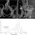
Echocardiography uses Doppler physics to determine blood flow velocities in the heart. Using the modified Bernoulli equation (Fig. 12.2), flow velocities are converted to pressure gradients partially because the conventional understanding of aortic valve hemodynamics was formulated in the pre-echocardiographic era. The accurate acquisition of velocity data is technically demanding and requires expertise and commitment to quality. Given that flow velocities as determined by Doppler techniques are angle dependent, alignment of the angle of the ultrasound beam as close as possible (<15°) to the direction of blood flow of the aortic jet is critical in minimizing the error intrinsic in the Doppler equation [10]. In practice this is gained by interrogating the aortic stenosis jet from multiple windows with a continuous wave (CW) Doppler probe (Fig. 12.3). The highest obtained velocity is reported, unless atrial fibrillation is present. Where moderate or greater aortic stenosis is present, a non-imaging probe should be used, which offers the smallest footprint and optimal signal-to-noise ratio. Careful attention is paid to signal optimization especially gain settings [11]. Severe aortic stenosis usually results in a flow velocity of >4 m/s [12]. The shape of the CW ejection signal also contains additional information. In mild or moderate aortic stenosis, the signal is triangular and peaks in the early part of systole, while in severe AS it is rounded and peaks in mid-systole[13] (Fig. 12.4).
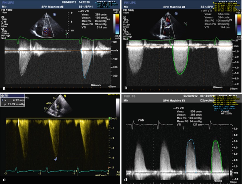
Fig. 12.2
The Bernoulli equation is used to derive the pressure gradient across a stenosis from proximal and distal flow velocities. The full Bernoulli equation includes convective acceleration, intentional, and frictional elements. In practice the frictional and inertial components are ignored, and the convective element is simplified by ignoring the proximal velocity to yield the more familiar ΔP = 4V 2, where ΔP is the pressure gradient and V is the maximal blood flow velocity across a stenosis, obtained using CW Doppler. When proximal velocities (V 1) are taken into account, a slightly fuller version of the simplified formula is rendered: ΔP = 4(V 1 2 – V 2 2). (From Anderson [10, p 195]. Reproduced with permission from MGA Graphics)
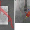
Fig. 12.3
Contrast this with the signal in Panel (a) where the patient has severe aortic stenosis with a peak velocity of 5.1 m/s, and a strong, rounded signal which peaks in mid-systole. Panel (b) shows a CW signal recorded from a patient with moderate aortic stenosis. The peak velocity is around 3.3 m/s, but importantly the signal shows peaking in the early part of systole. In panel (c), the patient has hypertrophic cardiomyopathy with dynamic sub-aortic obstruction. The signal is characteristically late peaking. Panel (d) shows a Doppler signal obtained from the right sternal border. The signal velocity from this window was highest than that obtained from the apex, resulting in a higher reported mean gradient and smaller calculated AVA
Fig. 12.4
Continuity equation. The continuity equation relies on the principle of conservation of mass. This means that flow in the LVOT must equal flow in the proximal aorta, distal to the aortic stenosis, i.e., SV1 = SV2. Given that flow is given by cross-sectional area (CSA) × velocity: CSA1 × VTI1 = CSA2 × VTI2. Solving for EOA aortic valve (or aortic valve area) yields the continuity equation. CSA1 cross-sectional area LVOT, VTI1 velocity time integral of LVOT, CSA2 effective orifice area of the aortic valve (EOA or AVA), VTI2 velocity time integral aortic stenosis jet (From Anderson [10, p 188]. Reproduced with permission from MGA Graphics)
Mean Pressure Gradient
Mean pressure gradient is one of the core measurements used to gauge aortic stenosis severity. Because mean pressure gradients reflect flow velocities at all time points during systole (in contrast to peak gradient), they may contain information incremental to the measurement of peak velocity. Like flow velocity, this measurement is flow dependent and can be misleading high in states of abnormally high or low flow (see below).
Aortic Valve Area (AVA)
Determination of AVA by the continuity equation provides a useful index of aortic stenosis severity in low- and high-flow states, although this measurement is also flow dependent to a degree. It relies on the principle of conservation of mass and is given by the formula AVA × VTIav = CSAlvot × VTIlvot (Figs. 12.4 and 12.5). When the equation is rearranged for AVA, the numerator of the equation is stroke volume across the valve. This is usually determined from an estimate of left ventricular outflow tract (LVOT) area which, when multiplied by the mean of flow velocities throughout systole in the LVOT (VTI or velocity time integral), yields stroke volume. Calculation of the LVOT area relies, in turn, upon and accurate linear assessment of the LVOT, which is obtained from a zoomed up, optimized view in the parasternal long-axis window (Fig. 12.1). The LVOT area is then calculated based on the assumption of a circular LVOT. The VTI in the LVOT is obtained using the pulse wave (PW) mode, with the sample volume positioned just proximal to the zone of flow acceleration, usually 5–10 mm ventricular to the aortic valve. An important principle is that the flow velocity should be sampled at the same point in space at which the LVOT dimension is measured. A detailed description of the technical requirements required to obtain these measurements is beyond the scope of this chapter but is well covered elsewhere [11]. Other measurements of stroke volume derived from volumetric assessment of the left ventricle by two- or three-dimensional techniques, or flow across other non-regurgitant valves (the right ventricular outflow tract for example), can occasionally be used. Once an estimate of stroke volume is obtained, the VTI of the highest-velocity transaortic signal obtained using CW mode is used to determine valve area. The continuity equation contains many assumptions and potential sources of error (see below) but works surprisingly well in clinical practice [14–17]. As with all hemodynamic measurements in aortic stenosis, accurate and reproducible results can only be obtained with superior sonographer training, a good understanding on the part of the echocardiographer of the errors and limitations intrinsic in the measurement and an overarching commitment to quality on the part of the echo lab.
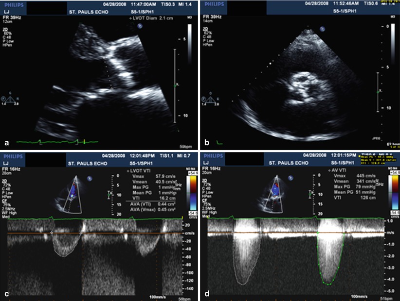
Fig. 12.5
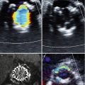
The core elements required for AS assessment by echo are illustrated here. Panel (a) is a zoomed in long-axis view which shows markedly thickened cusps. A measurement of the LVOT dimension has been made. Panel (b) shows the VTI of flow in the LVOT, obtained with PW Doppler. This measurement is required for calculation of aortic valve area using the continuity equation. Panel (c) shows the aortic valve in short-axis orientation. This shows severe anatomic aortic stenosis and provides a useful confirmation of the hemodynamic measurements. Panel (d) shows the typical CW spectral Doppler signal of severe AS, obtained from the apical window. The measurements in this instance indicate critical AS with a valve area of 0.4 cm2
Velocity Ratio
If an accurate assessment of the LVOT dimension is not obtained, the LVOT area cannot be calculated; hence, stroke volume across the LVOT cannot be determined. In this instance, the ratio of the flow velocity in the LVOT to the flow velocity of the aortic jet may be a useful alternative to the continuity equation. Aortic stenosis is considered severe when the ratio is 0.25 or less [16]. The velocity ratio ignores natural variation of LVOT area with body size and lacks extensive outcome data supporting its use as a decision-making tool.
Experimental Measurements
A variety of experimental measurements have been proposed as alternative indices of AS severity [18–20]. In general, these measurements have been designed to more accurately determine the hemodynamic burden of aortic stenosis or to be useful in low-flow states. Because these measurements lack sufficient outcome data and may be cumbersome in a working lab, they are generally used in a niche or research setting and not presently endorsed as primary clinical working tools.
Sources of Measurement Variability, Error, and Discrepancies
Gradients and Velocities
As indicated, the major potential source of error is the misalignment of the ultrasound beam to the aortic stenotic jet. Careful attention to appropriate gain settings to avoid spectral broadening and tracing the crisp outer border when measuring the CW velocity signal are important technical considerations. The anticipated coefficient of variation in an tertiary echo lab with repeated measurements of the same patient is of the order of 3 % for determining the maximum velocity of the aortic and LVOT signals and somewhat greater for the determination of the VTI [15]. The simplified Bernoulli equation represents an abbreviation of the full formula in that it ignores proximal velocity as well as other hydraulic variables (see Fig. 12.2). This means that if there is significant flow acceleration in the LVOT, the pressure gradients will be overestimated if the simplified version of the Bernoulli is used. This is easily accounted for mathematically by using the more complete formula when flow velocities in the LVOT are >1.5 m/s, at least in so far as peak gradients are concerned (Fig. 12.2).
Because peak LV and peak aortic pressure do not occur at the same point in time, the peak-to-peak gradient familiar to catheterizing cardiologists is a non-physiological measurement and is invariably less than the maximum instantaneous pressure difference which is reflected in the aortic jet velocity (Fig. 12.6). This can cause a discrepancy between the catheter-derived and echo-derived peak gradient in aortic stenosis. The mean gradients are typically comparable however.
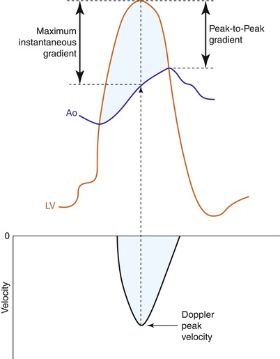
Fig. 12.6
The catheter-derived peak-to-peak gradient is compared to the Doppler-derived maximum instantaneous gradient in a patient with mild to moderate aortic stenosis. The Doppler measurement measures the gradient at the same time point in systole while the catheter gradient is a non-physiological measurement (From Anderson [10, p 198]. Reproduced with permission from MGA Graphics)
Pressure Recovery
Pressure recovery is a phenomenon that reflects the dynamic interplay between kinetic and potential energy across the aortic valve. During blood flow across the aortic valve, potential energy is converted into kinetic as flow velocity accelerates. Downstream from the stenosis, this is converted back into potential energy and pressure increases downstream [21]. The greatest pressure drop occurs at the level of the vena contracta of the stenotic jet where flow velocity is greatest; usually catheters are positioned downstream where recovery of pressure has occurred (Fig. 12.7). It is therefore not surprising that catheter-derived pressure gradients may be lower and Gorlin formula-derived valve areas higher than their echo-derived counterparts under certain circumstances [22]. Rapid pressure recovery is favored in patients with mild stenosis and small aortas [21] and is unlikely to be clinically important when the diameter of the aorta is >30 mm. Indices have been developed to account for the effects of pressure recovery; yet these are seldom used in clinical practice [18]. Notwithstanding, an awareness of the phenomenon is sometimes useful in resolving inconsistent or disparate results.
Fig. 12.7
The left hand panel indicates a situation where “normal” pressure recovery. The right hand panel indicates “rapid pressure recovery,” a situation favored by small aortas and small mechanical prosthetic valves. The gradient as measured by Doppler is derived from the maximum velocity (V 2) and will reflect the “unrecovered” or maximal pressure gradient. In the left hand panel, the hemodynamic catheter may be positioned in the zone between a and b, i.e., the “unrecovered zone” and hence significant disparity between echo and catheter gradients is unlikely to occur. In the right hand panel, the hemodynamic catheter may be positioned upstream, in the zone of recovered pressure, a scenario that may lead to a discrepancy in the gradient estimate between the two techniques (From Anderson [10, p 198]. Reproduced with permission from MGA Graphics)
Valve Area: Planimetry
The planimetered aortic valve area is derived by tracing a short-axis view of the aortic valve (Fig. 12.8). It represents peak geometric orifice area and will be greater than the continuity valve area or effective orifice area (EOA). The EOA represents the average vena contracta area throughout the cardiac cycle and more accurately represents hemodynamic load and outcome. Imaging difficulties caused by acoustic shadowing and reverberation artifacts can compromise accuracy, and this measurement is usually considered more accurate with TEE. Identifying the plane that incorporates the minimal orifice area can be problematic especially in bicuspid valves. 3D imaging is likely to prove useful in this setting [23].

Fig. 12.8
Planimetry of the aortic valve may be useful when Doppler data is unreliable or cannot be obtained. Geometric orifice area is obtained with this technique, as opposed to effective orifice area determined with the continuity equation. In this instance, a value of 0.9 cm2 for AVA is obtained. Effective orifice area represents the area of the vena contracta of the AS jet and is smaller than the geometric (or anatomic) orifice area. Planimetry measurements may be limited by acoustic artifacts, and care must be taken that the cut plane incorporates the smallest orifice area, a situation where 3-D imaging may be useful
Valve Area: Continuity Equation
The continuity equation depends on the ability to accurately calculate flow across the LVOT. The measurement subject to the highest variability is that of the LVOT dimension [15]. Given that this measurement is squared, the potential for measurement error and variability is high. In addition the assumptions that underpin the continuity equation are its “Achilles heel.” Specifically it assumes a circular LVOT geometry, which is untrue in some and, perhaps, most cases [24–26]. In particular, the LVOT shape can be distorted by abnormal basal septal hypertrophy or protruding mitral annular calcium. Another assumption is that of uniform velocity distribution of flow in the LVOT. It is known that the velocity profile in the LVOT may be distorted and skewed in conditions of high subvalvular flow such as aortic regurgitation (AR). It is likely that emerging 3D techniques will allow for more accurate estimation of LVOT flow velocities and geometry, hence reducing potential for variability error in AS assessment [25].
Classification and Reporting of Aortic Stenosis
The stenotic aortic valve represents one aspect of cardiac pathology and requires understanding in the context of other parameters of structure and function—including LV ejection fraction, diastology, LV mass, aortic and mitral regurgitation, and pulmonary artery pressure. As well as, describing the morphologic appearance of the aortic valve, the three core hemodynamic measurements—peak velocity, mean pressure, and aortic valve area—are reported. In addition, a sense of the correlation between the morphologic appearance and hemodynamic measurements, and an estimate of the reliability of the hemodynamic measurements, is often useful. To minimize measurement variability the same LVOT dimension should be used in valve area calculations in serial studies. Both aortic annulus and LVOT dimensions are reported in our lab. Similarly the window where the highest aortic jet velocity was obtained should be noted.
The traditional cut points for severe AS do not take account of body size, although it seems intuitive that a 1 cm2 valve area might be adequate for a small female with a body surface area of 1.4 cm2, but represent severe or critical aortic stenosis for a much larger individual with say a BSA of 2.5 m2 with higher cardiac output requirements. Most experts consider that it is appropriate to consider indexed valve areas in decision making in small individuals; the value is less established for larger persons. Indexed valve area cut points for mild, moderate, and severe AS have been published [11].
Related posts:
 Transcatheter Aortic Valve Replacement: Current Evidence from Large Multicenter Registries
 Positron Emission Tomography Evaluation of Aortic Stenosis
 Pathologic Findings in Aortic Stenosis
 Transcatheter Aortic Valve Replacement in Patients with Chronic Kidney Disease: Pre-procedural Assessment and Procedural Techniques to Minimize Risk for Acute Kidney Injury
 Aortoiliofemoral Assessment: MDCT
 Valve-in-Valve for Transcatheter Aortic Valve Replacement: Do Imaging Requirements Change?
Stay updated, free articles. Join our Telegram channel

Full access? Get Clinical Tree


