Chapter 2 Echocardiography
ECHOCARDIOGRAPHIC EXAMINATION
Two-Dimensional Transthoracic Examination
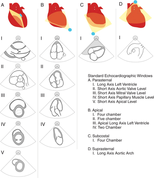
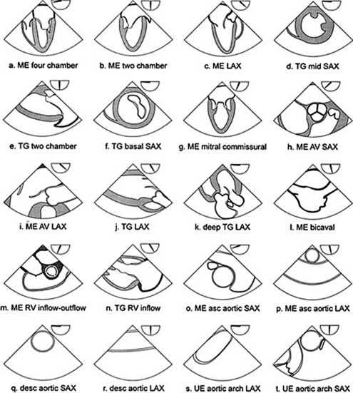
During the routine echocardiography examination, a fan-shaped beam of ultrasound is directed through a number of selected planes of the heart to record a set of standardized views of the cardiac structures for subsequent analysis. These views are designated by the position of the transducer, the orientation of the viewing plane relative to the primary axis of the heart, and the structures included in the image (Fig. 2-1).

FIGURE 2-1 Diagrammatic representation of the transducer position on the anterior surface of the chest with the corresponding standard echocardiographic windows.
Left Parasternal Imaging Planes
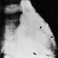
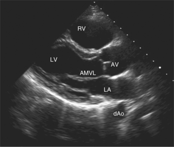
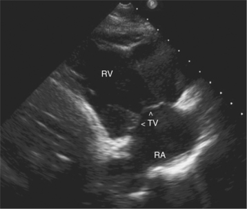
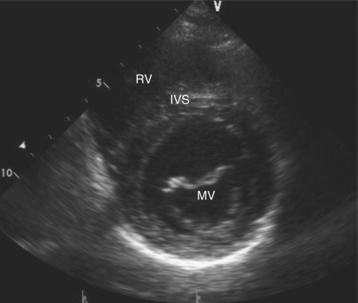
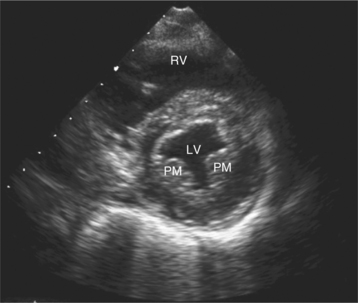
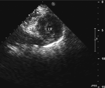
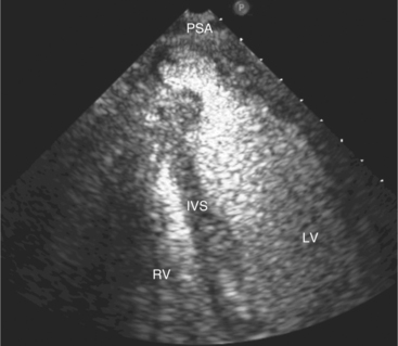
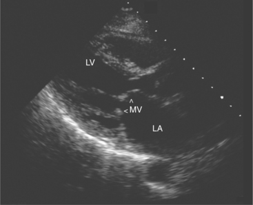
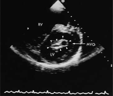
Parasternal views of the heart are obtained by positioning the transducer along the left parasternal intercostal spaces. From this position, long- and short-axis images of the heart can be obtained. In the long-axis view, the structures which can be assessed are mitral leaflets and chordal apparatus, right ventricular outflow tract, aortic valve, left atrium, long axis of the left ventricle, and aorta (Fig. 2-2). Rightward angulation allows more complete imaging of the right ventricle. The right ventricular inflow view allows assessment of the right atrium, the proximal portion of the inferior vena cava, and the entry of the coronary sinus, the tricuspid valve, and the base of the right ventricle (Fig. 2-3). The parasternal short-axis images of the heart are obtained as the transducer is rotated 90 degrees from the long-axis plane and swept from a cranial to a caudal position. The most cranial view allows visualization of the aortic valve, atria, right ventricular outflow tract, and proximal pulmonary arteries. The three normal coronary cusps of the aortic valve can be viewed with possible imaging of the proximal right coronary artery arising from the right coronary cusp at the 10 o’clock position, and the left main coronary artery originating from the left coronary cusp at the 3 o’clock position (Fig. 2-4). A series of cross-sectional images of the left and right ventricles are created by moving the transducer caudally. The right ventricle appears as a crescentic structure along the right anterior surface of the left ventricle. At the basal level, the fish-mouthed appearance of the mitral valve is apparent (Fig. 2-5). At the midventricular level, the anterolateral and posteromedial papillary muscles are seen (Fig. 2-6). The most caudal angulation allows visualization of the left ventricular apex (Fig. 2-7).

FIGURE 2-2 Two-dimensional parasternal echocardiographic view of the long axis of the left ventricle. In this diastolic image, the mitral valve leaflets are open and the aortic valve leaflets are closed. The descending aorta can be seen in cross section as it passes beneath the left atrium. AV, aortic valve; dAo, descending aorta; LA, left atrium; AMVL, anterior mitral valve leaflet; LV, left ventricle; RV, right ventricular outflow tract.

FIGURE 2-3 Two-dimensional parasternal echocardiographic view of the long axis of the right heart. The tricuspid valve leaflets (arrowheads) are seen closing in systole. RA, right atrium; RV, right ventricle; TV, tricuspid valve.

FIGURE 2-4 Two-dimensional parasternal short-axis view at the base of the heart. The aortic root with its three aortic sinuses is shown in the center with the left atrium directly posterior to it. A prominent left atrial appendage is present (long arrow), and the left upper pulmonary vein can be seen entering the left atrium. The right ventricular outflow tract lies anterior to the aorta, with the posterior cusp of the pulmonic valve depicted by the short arrow. LA, left atrium; LAA, left atrial appendage; PV, pulmonic valve; pv, pulmonary vein; RA, right atrium.

FIGURE 2-5 Two-dimensional parasternal short-axis view of the left ventricle at the level of the mitral valve. In diastole, the mitral valve leaflets are open in a “fish mouth” pattern. The left ventricle appears circular and the right ventricle is crescentic in shape. IVS, interventricular septum; MV, mitral valve; RV, right ventricle.

FIGURE 2-6 Two-dimensional parasternal short-axis view of the left ventricle at the level of the papillary muscles. Both papillary muscles can be seen projecting into the lumen of the left ventricle. LV, left ventricle; PM, papillary muscles; RV, right ventricle.
Apical Imaging Planes
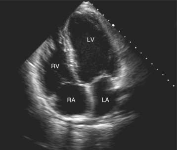
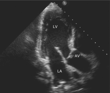
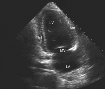
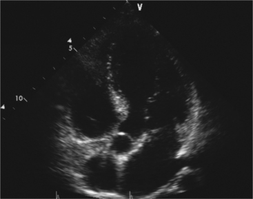
By placing the transducer at the cardiac apex and orienting the imaging sector toward the base of the heart, it is possible to obtain the apical views of the heart. This allows visualization of all chambers of the heart and the tricuspid and mitral valves. With the transducer oriented in a mediolateral plane at 0 degrees, an apical four-chamber view of the heart is obtained (Fig. 2-8). As the transducer is rotated 45 degrees clockwise to this plane, the apical long-axis view of the heart is obtained (Fig. 2-9), and further clockwise rotation of the transducer to a full 90 degrees produces the apical two-chamber view (Fig. 2-10). The apical two-chamber view is important because it allows direct visualization of the true inferior and anterior wall of the ventricle. Superficial angulation of the scanning plane from the apical four-chamber view brings the left ventricular outflow tract and aortic valve into view, producing the five-chamber view (Fig. 2-11).

FIGURE 2-8 Two-dimensional apical four-chamber echocardiographic view of the heart. To obtain this view, the transducer is placed at the cardiac apex. This produces an image in which the apex and ventricular chambers of the heart are at the top of the image sector and the atria are in the far field of the image. By convention, the left heart structures are positioned to the right of the image. LA, left atrium; LV, left ventricle; RA, right atrium; RV, right ventricle.

FIGURE 2-9 Two-dimensional apical long-axis view of the heart. To obtain this view, the transducer is rotated so that the index marker is pointed toward the suprasternal notch. AV, aortic valve; LA, left atrium; LV, left ventricle.

FIGURE 2-10 Two-dimensional apical two-chamber view of the heart. To obtain this view, the transducer is rotated 45 degree clockwise from the long-axis view. This image plane lies between long-axis view and four-chamber view. In this view, the true anterior (Ant) and inferior (Inf) walls can be seen. LA, left atrium; LV, left ventricle.
Subcostal Imaging Planes
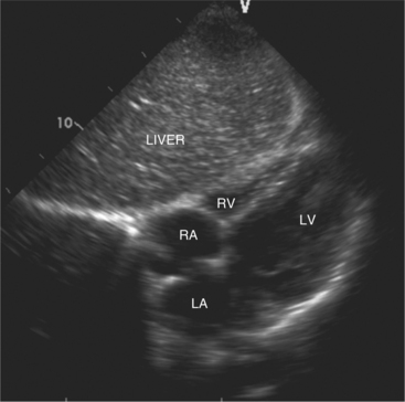
The subcostal window allows ultrasound access to the heart through the solid tissue of the liver, which readily transmits sound waves. The alignment of the heart relative to this approach permits better visualization of the atrial and ventricular septae because the sound beam strikes these structures in a perpendicular direction. A series of long- and short-axis images are usually obtained from this window. The inferior vena cava and hepatic veins, the liver, and the abdominal aorta can also be evaluated subcostally (Fig. 2-12). Facility with subcostal imaging is important because in some instances, as in the intensive care unit setting, it may be the only viewpoint from which to image the heart in the patient with chest wall injury, hyperinflated lungs, or pneumothorax. In infants and small children the subcostal window provides excellent images of all cardiac structures.
Suprasternal Imaging Planes
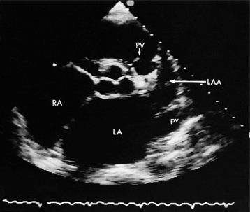
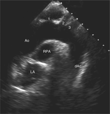
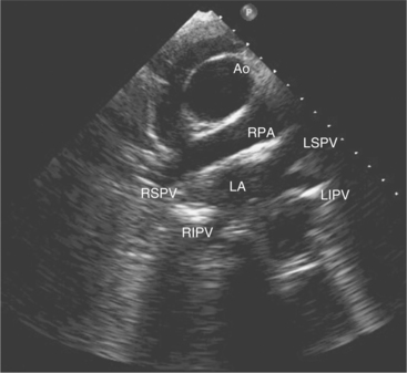
Suprasternal views are obtained by placing the transducer in the suprasternal notch. Both longitudinal and transverse planes of the great vessels can be imaged. The longitudinal plane orients through the long axis of the aorta and includes the origins of the innominate, left common carotid, and left subclavian arteries (Fig. 2-13). The transverse plane includes a cross section through the ascending aorta, with the right pulmonary artery crossing behind. Portions of the innominate vein and superior vena cava are visible anterior to the aorta. The left atrium and pulmonary veins are posterior to the right pulmonary artery (Fig. 2-14).

FIGURE 2-13 Two-dimensional suprasternal long-axis view of the aortic arch. The proximal portions of the brachiocephalic vessels are demonstrated arising from the aortic arch: (1) right brachiocephalic artery, (2) left common carotid artery, and (3) left subclavian artery. The right pulmonary artery (RPA) can be seen in cross section as it passes beneath the ascending aorta (Ao). DAo, descending aorta; LA, left atrium.

FIGURE 2-14 Two-dimensional suprasternal short-axis echocardiographic view of the aortic arch. The right pulmonary artery (RPA) crosses beneath the aorta (Ao) and the pulmonary veins enter the left atrium with a “crablike” appearance. LA, left atrium; LIPV, left inferior pulmonary vein; LSPV, left superior pulmonary vein; RIPV, right inferior pulmonary vein; RSPV, right superior pulmonary vein.
Right Parasternal Views
The right parasternal border may also be useful for viewing the heart in either transverse or longitudinal orientations. These views are particularly helpful with medially positioned hearts, right ventricular enlargement, and rightward orientation of the ascending aorta. By allowing direct visualization of the right atrium, both venae cavae, and the interatrial septum, this view is also of particular value in the assessment of interatrial shunt flow, and in the detection of anomalous pulmonary venous drainage.
Transesophageal Imaging
Transesophageal imaging is a valuable technique to visualize the heart and great vessels in patients with suboptimal transthoracic imaging windows. This may occur as a result of body habitus, lung disease, or operative room or intensive care environment where access to the chest wall and optimal positioning is prohibitive. Transesophageal imaging uses a specially designed ultrasound probe incorporated within a standard gastroscope. This semi-invasive procedure requires blind esophageal intubation. Because of the close proximity of the heart to the imaging transducer, high-frequency transducers (5.0 to 7.5 MHz) are routinely used, which allows better definition of small structures than the lower frequencies used transthoracically (2.5 to 3.5 MHz). Therefore, transesophageal imaging is particularly valuable in the routine clinical setting for the detection of atrial thrombi, small vegetations, diseases of the aorta, atrial septal defects, patent foramen ovale, and the assessment of prosthetic valve function. It is used in the operating or catheter suites to monitor and assess the repair of cardiac structures.
Current instrumentation allows imaging of multiple planes through the heart with multiplane transesophageal probes in which the ultrasound plane is electronically steered through an arc of 180 degrees. The anteroposterior orientation of images from the esophagus is the reverse of images from the transthoracic window because the ultrasound beam first encounters the more posterior structures closest to the esophagus (Fig. 2-15).

FIGURE 2-15 Diagrammatic representation of the standard imaging planes obtained with multiplane transesophageal echocardiography. Views from the upper esophageal, midesophageal, and transgastric probe orientations are demonstrated. The icon adjacent to each view indicates the approximate multiplane angle. AV, aortic valve; LAX, long axis; ME, midesophageal; RV, right ventricle; SAX, short axis; TG, transgastric; UE, upper esophageal.
(Reprinted with permission from the Journal of the American Society of Echocardiography from Shanewise JS, et al. ASE/SCA guidelines for performing a comprehensive intra-operative transesophageal echocardiographic exam, J Am Soc Echocardiogr 12:887, 1999.)
The Normal Doppler Examination
By applying the Doppler principle to ultrasound, the frequency shift of ultrasound waves reflected from moving red blood cells can be used to determine the velocity and direction of blood flow. This can be done with either pulsed Doppler or continuous wave Doppler. Pulsed Doppler allows analysis of the velocity and direction of blood flow at a specific site. Continuous wave Doppler allows resolution and analysis of high-velocity flow along the entire length of the Doppler beam. The data can be displayed graphically (Fig. 2-16). By convention, flow toward the interrogating transducer is represented as a deflection above, and flow away from the transducer appears as a deflection below the baseline. The x-axis represents time and the y-axis represents velocity.

FIGURE 2-16 Continuous wave Doppler spectral tracing of flow across the mitral valve from the apical window. In diastole, flow is recorded above the baseline as blood moves toward the transducer at the apex across the mitral valve into the left ventricle. In systole, mitral regurgitant flow is shown below the baseline as it passes away from the apex and into the left atrium. This patient with rheumatic mitral stenosis has high velocity mitral inflow (1.8 m/sec) and mitral regurgitation (5 m/sec).
Color-flow mapping also uses pulsed Doppler methodology, but it maps flow velocity at multiple sites within an area and overlays this information in color on a black-and-white two-dimensional image. By convention, color coding for flow velocity toward the transducer is red and flow velocity away from the transducer is blue. Higher velocities are mapped as brighter shades. A mosaic of color represents turbulent flow. Parallel alignment to flow is essential for accurate Doppler quantitation.
Parasternal Long-Axis View
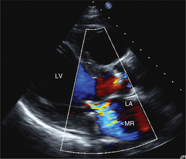
In this view, mitral regurgitation is seen as a discrete blue jet in the left atrium during systole (Fig. 2-17). Small jets can be seen with normal valves.

FIGURE 2-17 A parasternal long-axis view of the mitral valve in systole. A large stream of mitral regurgitation (MR) (arrowhead) is seen emerging from the leaflet coaptation point and spreading into the left atrium (LA). The jet is blue (indicating flow away from the transducer) with mosaic of color to reflect turbulent flow. LV, left ventricle.
Aortic regurgitation is seen as blue or red jet emanating from a closed aortic valve. The jet is located in the left ventricular outflow tract and occurs in diastole. The presence of this jet represents an abnormal aortic valve.
Right Ventricular Inflow View
Inferior vena cava inflow is seen as a red jet seen at the inferior margin of the right atrium. It has both systole and diastole phases and flow velocity is normally less than 1.0 m/sec by pulsed Doppler.
Tricuspid inflow is seen as red jet crossing the tricuspid valve. It occurs in diastole with velocities less than 0.6 m/sec. Tricuspid regurgitation is a blue jet in the right atrium which occurs in systole. Small jets are normal. The peak velocity of regurgitant flow can be quantified by continuous wave Doppler.
Parasternal Short Axis
Inferior vena cava inflow is a continuous low-velocity red jet that enters through the right atrial floor adjacent to the interatrial septum. Vigorous caval flow such as seen in children may be confused with left to right interatrial shunt flow. Pulmonary outflow is a systolic blue jet in the pulmonary artery.
The normal velocity across the pulmonary outflow tract is 0.6 to 0.9 m/sec in adults and 0.7-1.2 m/sec in children.
Apical Views
Transmitral and tricuspid flow are best evaluated in the four-chamber view as a result of the parallel position of the Doppler beam to the direction of blood flow. Likewise, transaortic flow can be assessed in the apical long axis or five-chamber view.
The flows detected in this view are:

FIGURE 2-18 Pulsed Doppler spectral profile of mitral inflow obtained from an apical window. Flow toward the transducer is shown above the baseline in diastole during left ventricular filling. The typical mitral biphasic-filling pattern is seen, with a prominent early filling wave (E wave) and smaller late diastolic filling wave (A wave).

FIGURE 2-19 Pulsed Doppler spectral profile of aortic outflow obtained from an apical window. Flow velocities are plotted below the baseline to indicate that the direction of flow is away from the apically positioned transducer. The typical aortic flow profile is a systolic flow with rapid upstroke to a peak velocity in midsystole and rapid decline in velocity during late systole.
Other Views
Subcostal views are useful for assessing flow within the inferior vena cava, hepatic veins, and abdominal aorta. The suprasternal window is used for recording flow in the ascending and descending aorta and in the superior vena cava.
Myocardial Doppler Tissue Imaging
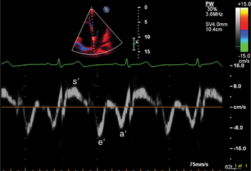
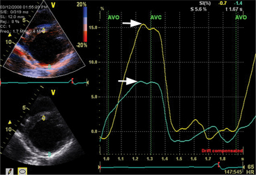
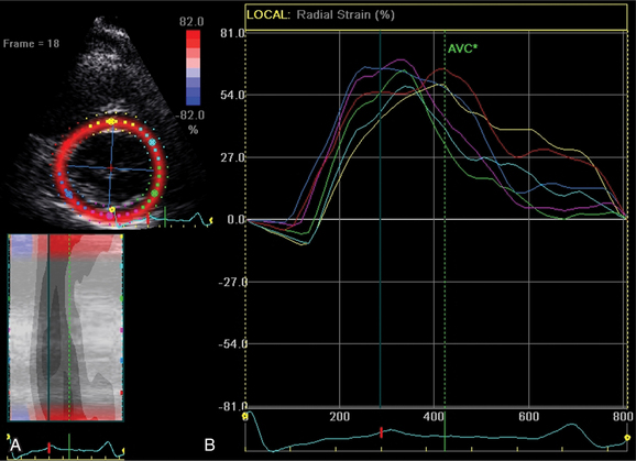
The transducer properties can be manipulated so that myocardium (low velocity) is the target of ultrasound reflection rather than blood cells (high velocity). Similar Doppler principles can be applied with color saturation of the tissue to indicate direction and velocity of the myocardium. A sample volume (similar to pulsed Doppler) is placed within the myocardium or valvular annulus to obtain a quantitative spectral profile of myocardial motion (Fig. 2-20). From the fundamental parameter of velocity, strain or strain rate imaging that measures tissue deformation can be derived (Fig. 2-21). Dopplerderived tissue velocity, strain and strain rate have been demonstrated to improve evaluation of myocardial mechanics when compared to previous measures such as wall thickening or motion.

FIGURE 2-20 Tissue Doppler imaging shows myocardial velocity in a target sample region. In this case the sample volume is placed at the septal mitral annulus. The systolic motion of the annulus (s′) and the diastolic motion (e′ and a′) are shown.

FIGURE 2-21 Tissue velocity derived radial strain of the left ventricle shown from the midventricular short axis. The two areas of interest are shown by ovals superimposed on the myocardium. The peak strain value for normal myocardium (anteroseptum, yellow curve) has a higher positive strain (myocardial lengthening) than dysfunctional myocardium (inferior wall, green curve) during systole.
Novel Echocardiographic Tools
Contrast Echocardiography
Contrast echocardiography uses intravenous agents that result in increased echogenicity of blood or myocardium with ultrasound imaging.
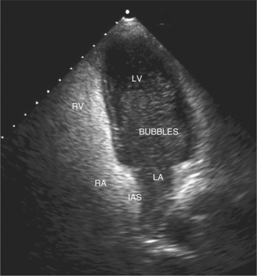
Contrast agents form small microbubbles, which at low ultrasound power, output disperse ultrasound at the gas and liquid interface, thus increasing the signal detected by the transducer. Right heart contrast is performed with injection of agitated saline and enables detection of right to left intracardiac shunts (Fig. 2-22). Left heart contrast agents consist of air or fluorocarbon gas encapsulated with stabilizing substances such as denatured albumin or monosaccharides. The microbubbles that are formed are small enough to pass through the pulmonary capillary bed, thus allowing opacification of the left heart following intravenous injection. The opacification of left ventricular cavity enhances endocardial border and cardiac mass identification particularly in cases of suboptimal acoustic windows (Fig. 2-23). Contrast echocardiography improves analysis of regional wall abnormalities. Real-time myocardial contrast echocardiography is being investigated as a tool for quantitative analysis of myocardial perfusion.

FIGURE 2-22 Apical four-chamber view recorded after the injection of agitated saline into an upper limb vein. Agitated saline contrast is seen to fill the right atrium (RA) and right ventricle (RV) before entering the left atrium (LA) and left ventricle (LV). The image is acquired after a Valsalva maneuver that transiently increases the right atrial pressure. This is reflected in the leftward displacement of the interatrial septum (IAS) resulting in increased right to left flow through the patent foramen ovale.

FIGURE 2-23 Apical four-chamber view recorded of a patient with left ventricular apical pseudoaneurysm (PSA) following left ventricular contrast agent injection showing complete cavity opacification and delineation of all left ventricular walls. IVS, interventricular septum; LV, left ventricle; RV, right ventricle.
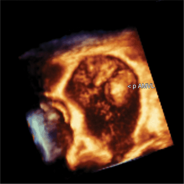
Three-Dimensional Echocardiography
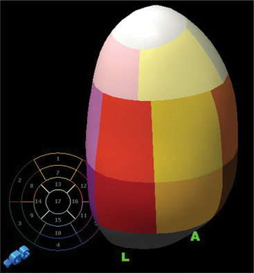
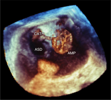
Volumetric imaging using a complex multi-array transducer to acquire three-dimensional pyramidal volume data is used to obtain images of the cardiac structures in three spatial dimensions. The structures may be viewed as a three-dimensional image or displayed simultaneously in multiple two-dimensional tomographic image planes. Postacquisition processing involves cropping that allows different views of the interior structures of the heart to be displayed. The structure studied can be manipulated so that it is viewed from multiple angles such as the surgical enface view of the mitral valve from the left atrium (Fig. 2-24). Quantitative volumetric data obtained by tracing the endocardial borders increases the accuracy of left ventricular volume assessment and allows for assessment of the right ventricular shape and volume (Fig. 2-25). Real-time three-dimensional transesophageal echocardiography (TEE) is currently being used to assist with device implantation in the catheter laboratory (Fig. 2-26). The current limitations of this technique, which is continually improving, include image quality, ultrasound artifact, and temporal resolution.

FIGURE 2-24 A three-dimensional enface view of the mitral valve from the left atrial perspective. There is prolapse of the middle scallop of the anterior mitral leaflet (pAMVL).

FIGURE 2-25 A three-dimensional left ventricular volume assessment allows all regions of the ventricular myocardium to be incorporated into the volume assessment. Each region is depicted by the different color code representing the 17-segment model. The image is from a patient with dilated cardiomyopathy and thus the ventricular shape is more globular in structure.

FIGURE 2-26 A three-dimensional study recorded during an atrial septal defect closure procedure. The image is recorded from the left atrial aspect showing the catheter traversing the atrial septal defect (ASD). The Amplatzer Atrial Septal Closure device (AMP) is seen at the tip of the catheter (CATH) as it is being positioned along the interatrial septum.
Two-Dimensional (Speckled) Strain Echocardiography
A new measure of myocardial strain analyzes motion by tracking speckles in the ultrasound image of the myocardium in two dimensions. The geometric shift of each speckle represents focal myocardial deformation. Software is available to process the temporal and spatial information and thus by tracking the speckles, two-dimensional tissue velocity, strain, and strain rate can be calculated. This technique, unlike Doppler measurement of strain, is not angle dependent (Fig. 2-27).

FIGURE 2-27 Two-dimensional radial speckle strain calculated from a short axis recording at the level of the mitral annulus. On the top left (A), the left ventricular short-axis view with the region of interest divided into six color-coded segments is displayed. The right panel (B) shows the graphical representation of the radial strain of all accepted segments. The myocardium thickens during systole and hence there is a positive deflection in the value of radial strain during systole.
Evaluation of Cardiac Chambers
Normal Linear Dimensions
By convention, most laboratories report the size of the left atrium, aortic root, and left ventricle from the measurement of the linear dimensions of each structure in the parasternal long-axis view of the heart (Table 2-1). All linear dimensions have been shown to bear a direct linear relation to body height. Normal chamber dimensions have also been determined for each of the standard two-dimensional views to allow quantitative assessment of each chamber or great vessel from any view.
TABLE 2-1 Normal linear dimensions*
Aortic root—end diastole | 24-39 mm |
Left atrium—end systole | 25-38 mm |
Left ventricle—end diastole | 37-53 mm |
Interventricular septal thickness—end diastole | 7-11 mm |
Left ventricular posterior wall thickness—end diastole | 7-11 mm |
Left Ventricular Volume
There are a number of methods for calculating left ventricular volume from two-dimensional echocardiographic images that require the assumption of a geometric shape of the left ventricle (Fig. 2-28).

FIGURE 2-28 Diagrammatic representations of the left ventricle showing the geometric models that have been used to calculate left ventricular volume. The shaded figure indicates the true chamber volume with the superimposed solid figure demonstrating the geometric shape described by the formula. The Simpson’s rule method comes closest to approximating the true shape of the ventricle. A, area; D, diameter; L, length; LAX, long axis length; LVID, left ventricular internal dimension.
Rights were not granted to include this figure in electronic media. Please refer to the printed book.
(From Weyman AE: Principles and Practice of Echocardiography, ed 2, Philadelphia, 1994, Lea & Febiger.)
The ellipsoid formula requires measuring the length of the ventricle and its diameter at the base. This volume estimation is valid in normal (symmetric) left ventricles, but it is less reliable when there is a distortion of ventricular shape (e.g., following myocardial infarction).
Simpson’s rule requires measuring the length of the ventricle from apical views and then determining the volume of a predefined number of disklike cross-sectional segments from base to apex.
Three-dimensional volume measurement makes no geometric assumptions and thus can determine the volume of both normal and distorted ventricles (see Figure 2-25).
Left Ventricular Systolic Function from Two-dimensional Images
Real-time echocardiographic assessment of endocardial motion and the degree of wall thickening during systole allows excellent qualitative assessment of global and regional ventricular function. Using this method, systolic function can be described as either normal or depressed, and regional function is either normal, hyperkinetic, hypokinetic, akinetic, or dyskinetic.
Quantitative assessment of ventricular function is available by estimating the global ejection fraction, determined by calculating the change in volume of the ventricle between diastole and systole.
The simplest method of estimating ejection fraction is to assume that the change in area at the base of the ventricle is representative of global ventricular function. In this way:
where LVIDD = the internal diameter of the base of the ventricle in diastole, and LVISD = the internal diameter of the ventricle in systole. Because this formula fails to account for apical function, 10% is empirically added if function at the apex is normal, 5% is added if the apex is hypokinetic, and 5% to 10% is subtracted if the apex is dyskinetic. The development of automated endocardial border detection now makes it possible to obtain an online estimate of ejection fraction based on changes in cavity area.
You can also estimate the ejection fraction by assessing the change in ventricular volume during the cardiac cycle using a simple formula, which assumes that the left ventricle is spherical:
Methods that estimate ejection fraction based on a single dimension obtained at the base of the heart, however, tend to overestimate global function in patients with apical infarction, and underestimate global function in patients with inferior basal infarctions.
Simpson’s rule generally provides a more accurate estimate of ejection fraction because it removes some of the assumptions about ventricular geometry. With current echocardiographic instrumentation, online and offline measurement capabilities provide easy access to this quantitative method. To perform the Simpson’s rule calculation, outline the full ventricular contour from the apical view in diastole. The automated measurement package will then draw a midline between the ventricular apex and the midpoint of the mitral annular plane and divide the ventricle into a series of small parallel disks of equal height, which run perpendicular to the midline. Because the radius and height of each disk is known, the volume of each disk can be computed. Summing the volume of each disk allows calculation of the diastolic ventricular volume. The same process is repeated for the end-systolic ventricular volume, and the ejection fraction is calculated as the difference in volume from diastole to systole, divided by the diastolic volume. The major limitation in this method is the inability to image the complete endocardial surface or the true length of the ventricle in some patients. The accuracy can be improved by using the biplane Simpson’s method, which averages the estimates of ventricular volume, obtained in orthogonal planes from apical four-chamber views and apical two-chamber views.
Two-dimensional echocardiographic estimates of ejection fraction make a number of assumptions about ventricular shape; they are most useful in normal or symmetrically dilated hearts. The application of three-dimensional technology can overcome the problems of estimating left ventricular ejection fraction in distorted ventricles.
Left Ventricular Systolic Function from Doppler Echocardiography
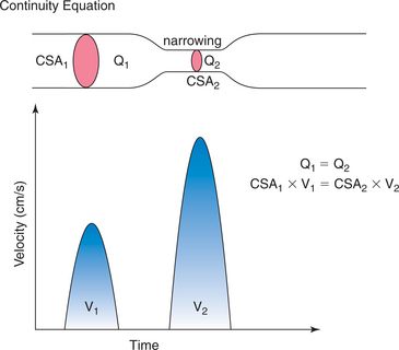
Doppler echocardiography makes it possible to estimate stroke volume and cardiac output by measuring volumetric flow through the heart. Stroke volume is calculated by measuring the cross-sectional area of a vessel or valve and then integrating the flow velocities across that specific region in the vessel or valve throughout the period of flow. The product of stroke volume and heart rate then gives an estimate of cardiac output (Fig. 2-29).

FIGURE 2-29 The Continuity equation for a region of narrowing is based on the volumetric flow on each side of the narrowing being equal (Q1 = Q2). The flow rate is equal to the product of the mean velocity and the cross sectional area. Thus CSA1 × V1 = CSA2 × V2. The mean velocity increases to maintain a constant flow rate through a region of narrowing. CSA1, the area of the lumen of the cylinder; CSA2, area of the stenosis; V1, velocity; V2, velocity of flow through the stenotic region.
Although cardiac output can be determined from the pulmonary, mitral, or tricuspid transvalvular flows, the aortic valve diameter and flow velocities are the most accurate. Further, there is excellent correlation between Doppler and roller pump estimates of stroke volume. In clinical practice, inaccuracies in measurement of the area of the outflow tract limit the use of Doppler estimates of cardiac output. This technique is successful, however, in following relative changes in cardiac output following pharmacologic intervention because the area of the outflow tract is assumed to remain constant.
Left Ventricular Diastolic Function
Impairment of left ventricular diastolic filling has been increasingly recognized as a clinical problem, either in association with systolic dysfunction or as an isolated entity. Two-dimensional echocardiography assesses left ventricular size, volumes, ejection fraction, and hypertrophy. The presence of an enlarged left atrium is found in more than 90% of patients with diastolic dysfunction.
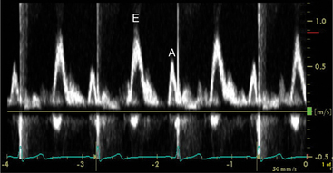
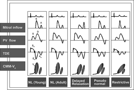
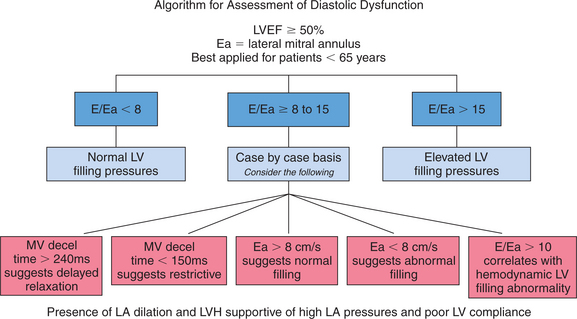
Echocardiographic Doppler assessment of left ventricular filling properties includes transmitral velocity and pulmonary vein flow characterization. Measurements of peak early (E) and late (A) diastolic flow velocities, isovolumic relaxation time, and deceleration time of early diastolic filling are all useful measures of diastolic function, but are limited by reduced accuracy for detection of high left atrial pressure in patients with normal ejection fraction or left ventricular hypertrophy, and poor ability to separate the effects of preload from relaxation. Flow propagation velocity by color M-mode and diastolic myocardial velocity by tissue Doppler (Ea) are measurements of diastolic function/impaired relaxation that are independent of the effects of preload. Flow propagation velocity relates inversely with the time constant of left ventricular relaxation. However, it can be difficult to measure and thus is less reproducible and may give erroneous results in patients with concentric left ventricular hypertrophy, small left ventricular cavity, and high filling pressures. Annular velocity is an index of myocardial relaxation and multiple studies have shown the ratio of transmitral E velocity to annular velocity Ea relates well with mean pulmonary capillary wedge pressure. However, it is a regional index and thus can vary between sampling sites and in patients with abnormal regional wall motion. The typical patterns observed with each of these methods in various forms of diastolic dysfunction are depicted in Fig. 2-30. A simplified algorithm for the use of E/Ea ratio in the clinical assessment of diastolic function is shown in Fig. 2-31. In addition, all diastology quantification measurements are not applicable for patients not in sinus rhythm or for those who have inflow obstruction (mitral stenosis, prosthetic valves).

FIGURE 2-30 Diagrammatic representation of Doppler transmitral flow velocities, pulmonary venous flow velocities, tissue Doppler velocity patterns, and color flow propagation in various states of left ventricular diastolic dysfunction. CMM-Vp, color M-mode velocity of propagation; PV, pulmonary venous flow; TDE, tissue Doppler echocardiography.
(Reproduced with permission from J.D. Thomas, MD.)

FIGURE 2-31 A suggested clinical algorithm for assessment of diastolic dysfunction for patients with normal systolic function (LVEF ≥ 50%). The assessment is integrated from tissue Doppler velocities at the mitral annulus (Ea), mitral inflow E velocity (E), mitral valve deceleration time and two-dimensional assessment of the left atrium (LA) and left ventricle (LV). LVEF, left ventricular ejection fraction; LVH, left ventricular hypertrophy; MV, mitral valve.
(Reproduced with permission from J. Hung, MD.)
Left Atrium
It is conventional to measure the anteroposterior dimension of the atrium at end systole in the parasternal long-axis view from a line drawn through the plane of the aortic valve. Measurement of the medio-lateral dimension and supero-inferior dimension can be made from the apical four-chamber view. Atrial enlargement may occur as a consequence of either an increase in atrial pressure (resulting from mitral stenosis or elevated left ventricular end-diastolic pressure), an increase in volume (as in mitral regurgitation), or as a consequence of primary atrial dysfunction (as in atrial fibrillation).
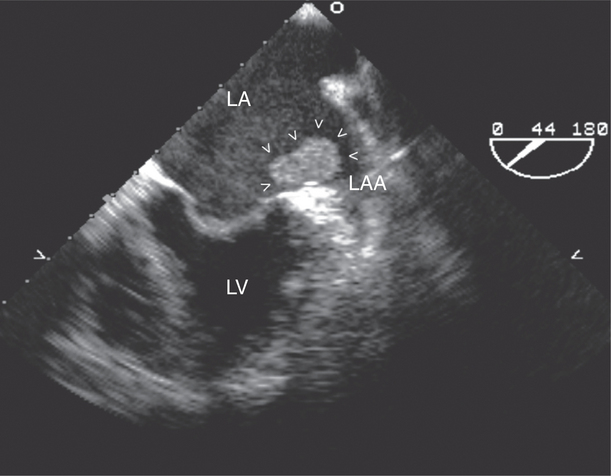
The left atrial appendage is a “dog ear”-shaped extension of the atrium situated along the lateral aspect of the chamber near the mitral annulus. Although usually inconspicuous, it is easily visible in the parasternal short-axis and apical two-chamber views of the atria when there is a dilated left atrium. Definitive imaging of the atrial appendage is usually performed with transesophageal imaging for the most accurate visualization of thrombus. It is important to realize that the appendage is a trabeculated structure. These trabeculae may be confused with thrombus, which may form within the appendage (Fig. 2-32).
Right Ventricle
Morphologically, the right ventricle can be divided into an inflow portion that includes the heavily trabeculated body of the ventricle, and an outflow portion that includes the infundibulum. The inflow portion extends from the tricuspid valve to the apex. The right ventricle generally has a crescentic shape when viewed in short axis, with its medial border formed from the convexity of the interventricular septum. The lateral or free wall of the right ventricle normally has a radius of curvature approximately equal to the left ventricular free wall. Because of the complex shape of the right ventricle, it is less amenable to geometric modeling than the left ventricle. Therefore, although there are simple, valid two-dimensional echocardiographic criteria for estimating right ventricular volume in nondistorted hearts, newer three-dimensional echocardiographic techniques are more reliable in assessing right ventricular volume.
Right ventricular enlargement may occur as a consequence of right ventricular volume loading, right ventricular infarction, or as part of a generalized cardiomyopathic process. In each instance, as dilatation progresses, the anteroposterior dimension of the ventricle increases and interventricular septal motion becomes increasingly abnormal. Specifically, in diastole the septum may appear to flatten, especially at the base, and in early systole the septum may move rightward (paradoxically) rather than leftward.
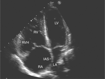
Pressure loading of the right ventricle results in progressive hypertrophy (Fig. 2-33). This may be difficult to discern with confidence because of the degree of trabeculation of the chamber. A free wall thickness of greater than 5 mm is a quantitative criterion for right ventricular hypertrophy. Marked pressure overloading typically produces systolic flattening of the interventricular septum.

FIGURE 2-33 Apical four-chamber view of a patient with severe primary pulmonary hypertension. The right ventricle (RV) is enlarged. There is hypertrophy of the free wall (RVH). The right atrium (RA) is enlarged and high right atrial pressures cause displacement of the interatrial septum (IAS) to the left. The left atrium (LA) and left ventricle (LV) are underfilled as a result of the reduced output from the right heart and are thus small.
Right Atrium
Assessment of right atrial size is usually made qualitatively by comparing it to the left atrium in the apical four-chamber view and quantitatively by measuring the maximal mediolateral and supero-inferior dimensions in this view. There are several normal structures within the right atrium. These include the Eustachian valve, which crosses from the inferior vena cava to the region of the foramen ovale, and the crista terminalis. In the apical four-chamber view, the crista can be seen as a ridge of tissue that separates the smooth-walled portion of the right atrium from its trabeculated anterior portion, often noted as a small mass of echoes located adjacent to the superior border of the right atrium. The right atrial appendage is a broad-based triangular structure that lies anterior to the atrial chamber near the ascending aorta. It is most visible in the parasternal views of the right atrium and readily visualized by TEE.
EVALUATION OF VALVULAR HEART DISEASE
Mitral Valve Disease
Mitral Stenosis
Echocardiography assists with the diagnosis and timing of intervention for mitral stenosis by providing accurate assessment of valve area, valve morphology, and the degree of pulmonary hypertension.
Acquired mitral stenosis is almost invariably caused by scarring and inflammation of the valve and chordal apparatus from past rheumatic fever. As a consequence of the disease, the mitral leaflets and chordal apparatus become diffusely thickened. Subsequently the valvular apparatus may shorten, fuse together at the commissural margins, and finally calcify. This results in a reduction in leaflet excursion so that the mitral leaflets appear to dome during diastole (Fig. 2-34). As the degree of valvular obstruction increases, flow through the valve decreases, left atrial pressure begins to rise, left atrial size increases (in the apical views, the interatrial septum is seen to bow to the right), and the potential for atrial thrombus formation is increased. Typically, the left ventricular size is normal or even small. If there is severe mitral stenosis, there may be paradoxical motion of the interventricular septum as a consequence of slow ventricular filling. Further, if there is pulmonary hypertension, the right heart and the pulmonary arteries may dilate and there may be severe tricuspid regurgitation. Almost all of these morphologic features are evident from the parasternal long-axis view of the heart; however, parasternal short-axis images are essential for planimetry of the mitral valve orifice (Fig. 2-35).

FIGURE 2-34 Parasternal long-axis echocardiographic view in a patient with rheumatic heart disease demonstrating marked calcification of the mitral valve leaflet tips. Instead of opening widely, the leaflets dome in diastole and the mitral orifice is severely restricted (arrowheads). LA, left atrium; LV, left ventricle; MV, mitral valve.

FIGURE 2-35 Parasternal short-axis echocardiographic view of the right and left ventricles at the mitral valve level. The mitral valve leaflets are thickened and the valve orifice is eccentrically restricted (arrowheads). The medial commissure is more tightly fused than the lateral commissure resulting in a larger orifice along the lateral aspect of the valve. LV, left ventricle; MVO, mitral valve orifice; RV, right ventricle.
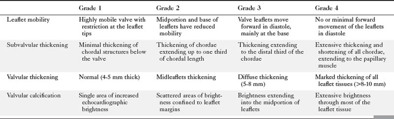
Echocardiographic grading of the severity of mitral stenosis is possible by assessing the degree of leaflet thickening, calcification, mobility, and the degree of chordal thickening and shortening (Table 2-2). When systematically graded, a low value of 1 to a high value of 4 is given for each of these characteristics. It is then possible to derive a numeric “score” that describes the extent of the mitral valve disease. This system is helpful in predicting the likelihood of successful balloon dilatation of the valve, with scores greater than 8 predicting a poor outcome following percutaneous dilatation.
Direct planimetry of the valve orifice in the short-axis plane can provide an accurate measurement of the mitral valve area. Three-dimensional echocardiography can improve the accuracy of detecting the smallest mitral orifice by providing simultaneous, perpendicular on axis views of the valve orifice.
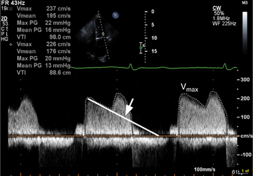
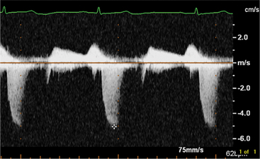
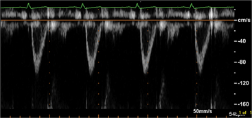
Continuous wave Doppler can help assess the severity of mitral stenosis because it enables calculations of the peak and mean transmitral gradients and the mitral valve area. For this purpose, the apical four-chamber view is preferable so that the Doppler beam can be directed through the mitral valve plane, parallel to the direction of left ventricular inflow. In contrast to the Doppler profile through a normal mitral valve, the continuous wave Doppler signal in patients with mitral stenosis demonstrates an increased velocity of flow in early diastole, with a prolonged descent of the early filling wave (deceleration time) that may merge into the late filling wave (Fig. 2-36). In patients with atrial fibrillation, the A wave, which reflects atrial contraction, is absent. The degree of prolongation of the phase of early filling relates directly to mitral valve area and to the severity of mitral stenosis.

FIGURE 2-36 Parameters that can be measured from the continuous wave Doppler assessment of the mitral valve include the mean pressure gradient and the mitral valve area from the pressure half-time measurement. Integration of the overall pressure gradient beneath the spectral display will calculate the mean pressure gradient (dotted curve). For the pressure half-time method, the time required for the pressure to decay from its peak value to one half of that value is determined. The velocity at which the pressure gradient has declined to one half of its peak can be calculated as 0.7 × Vmax. The time taken for this velocity to be reached is the pressure half-time (Pt1/2), which can be entered into the equation Mitral Valve Area = 220/Pt1/2.
Once you obtain the continuous wave Doppler profile, it is possible to calculate the transmitral gradient by converting the velocity information provided by the Doppler signal into an estimate of pressure using the simplified Bernoulli equation. In essence, the Bernoulli theorem states that the velocity (V) of flow across a stenosis relates to the pressure difference (P) across the stenosis. Specifically, the simplified Bernoulli equation predicts that the pressure gradient across a valve approximates a value four times the square of the velocity of flow across the valve (P = 4V2). Knowing the peak velocity of flow across the mitral valve, therefore, enables calculation of the peak pressure gradient across the valve. Similarly, the average of the velocities throughout all of diastole yields the mean gradient. Most commercial echocardiographic Doppler equipment contains software that can automatically integrate the velocity profile once it is traced, and then calculate the mean gradient using the Bernoulli equation. In general, the gradient across the mitral valve obtained by Doppler correlates well with that obtained at catheterization.
Doppler estimates of mitral valve area rely on the observation that the degree of prolongation of early filling relates directly to the degree of mitral stenosis. Quantification of this is possible by calculating the time for the pressure gradient across the mitral valve to fall to half its peak value, the pressure half-time. Pressure half-time is obtained from the continuous wave Doppler profile by determining the velocity half-time, measuring the time interval between peak transmitral velocity and the point where transmitral velocity has fallen to half its peak value.
In normal subjects, the pressure half-time is less than 60 ms. In contrast, in patients with mitral stenosis the half-time is usually in excess of 200 ms, with higher values in patients with more severe disease. An empirical formula that relates pressure half-time to the mitral valve area is as follows: Area = 220/Pressure Half-Time. This is fairly accurate compared with estimates of valve area determined by catheterization. From this empirical formula, patients with a pressure half-time of greater than 220 ms have a mitral valve area equal to or less than 1.0 cm2.

Full access? Get Clinical Tree

