Electron Beam Therapy


Electron Beam Therapy


High-energy electrons have been used in radiation therapy since the early 1950s. Originally, the beams were extracted mostly from betatrons, although a few linear accelerators and Van de Graaff generators with relatively low electron energies were also available. In the 1970s, high-energy linear accelerators, having photon and multienergy electron beam capabilities, became increasingly available for clinical use. The surge in the commercial development of these machines was prompted largely by the clinical experience gained at a few major centers, which showed that in some commonly encountered situations “there is no alternative treatment to electron beam therapy” (1).

The most clinically useful energy range for electrons is 6 to 20 MeV. At these energies, the electron beams can be used for treating superficial tumors (<5 cm deep) with a characteristically sharp dropoff in dose beyond the tumor. The principal applications are (a) the treatment of skin and lip cancers, (b) chest wall irradiation for breast cancer, (c) administering boost dose to nodes, and (d) the treatment of head and neck cancers. Although many of these sites can also be treated with superficial x-rays, brachytherapy, or tangential photon beams, the electron beam irradiation offers distinct advantages in terms of dose uniformity in the target volume and in minimizing dose to deeper tissues.

This chapter is intended to provide basic information on electron beam characteristics, dosimetry, and treatment planning. Most of the discussion will pertain to 6- to 20-MeV electrons, although the data at these energies can be qualitatively extrapolated to the lower or the higher energy range.


14.1. ELECTRON INTERACTIONS

As electrons travel through a medium, they interact with atoms by a variety of processes owing to Coulomb force interactions. These processes include (a) inelastic collisions with atomic electrons (ionization and excitation), (b) inelastic collisions with atomic nuclei (bremsstrahlung), (c) elastic collisions with atomic nuclei (nuclear scattering), and (d) elastic collisions with atomic electrons (electron-electron scattering).

In inelastic collisions, some of the kinetic energy is lost as it is used in producing ionization and excitation or converted to other forms of energy such as bremsstrahlung photons. In elastic collisions, kinetic energy is not lost, although it may be redistributed among the particles emerging from the collision. In low-atomic-number media such as water or tissues, electrons lose energy predominantly through ionization/excitation events with atomic electrons. In higher-atomic-number materials, such as lead, bremsstrahlung production is more important. In the collision process with the atomic electrons, if the kinetic energy acquired by the stripped electron is large enough for it to cause further ionization, the electron is known as a secondary electron or a δ-ray. As a beam of electrons travels through a medium, the energy is continually degraded until the electrons reach thermal energies and are captured by the surrounding atoms.

Multiple elastic collisions of a high-energy electron (multiple scattering) produce multiple small angle deflections. As a result, the electron follows a tortuous (zigzag) path, while it also continuously loses kinetic energy through inelastic collisions with atoms (ionization and excitation) until all of its kinetic energy is gone.


A. RATE OF ENERGY LOSS

An electron traveling in a medium loses energy as a result of collisional and radiative processes. The magnitudes of the two effects for water and lead are shown in Figure 14.1. Although the
theoretical treatment of this subject is given elsewhere (2, 3, 4, 5), it will suffice here to provide some important generalizations.


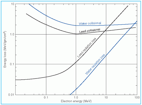
Figure 14.1. Rate of energy loss in MeV per g/cm2 as a function of electron energy for water and lead. (From Johns HE, Cunningham JR. The Physics of Radiology. 3rd ed. Springfield, IL: Charles C Thomas; 1969, with permission.)


A.1. Collisional Losses (Ionization and Excitation)

(a) The rate of energy loss depends on the electron density of the medium. (b) The rate of energy loss per gram per centimeter squared, which is called the mass stopping power, is greater for low-atomic-number (Z) materials than for high-Z materials (compare the water curve to the lead curve in Fig. 14.1). There are two reasons for this: First, high-Z materials have fewer electrons per gram than low-Z materials have and, second, high-Z materials have more tightly bound electrons, which are not as available for this type of interaction. (c) As seen in Figure 14.1, the energy loss rate first decreases and then increases with increase in electron energy with a minimum occurring at about 1 MeV. Above 1 MeV, the variation with energy is very gradual. (d) The rate of energy loss of electrons of energy 1 MeV and above in water is roughly 2 MeV/cm.


A.2. Radiation Losses (Bremsstrahlung)

The rate of energy loss per centimeter in a medium due to bremsstrahlung is approximately proportional to the electron energy and to the square of the atomic number (Z2). Moreover, the probability of radiation loss relative to the collisional loss increases with the electron energy and with Z. That means that x-ray production is more efficient for higher-energy electrons and higher-atomic-number absorbers.


A.3. Polarization

A high-energy electron loses more energy per gram per square centimeter in a gas than in traversing a denser medium, because of appreciable polarization of the condensed medium (5, 6, 7). Atoms close to the electron track screen those remote from the track. This phenomenon is particularly important in dosimetry with ionization chambers when energy deposition in a medium and a gas cavity are compared. The ratio of mass stopping power of water to air varies with electron energy, and consequently, the dose conversion factor for an air ionization chamber reading in water (or another condensed medium) varies with depth.


A.4. Stopping Power

The total mass stopping power (S/ρ)tot of a material for charged particles is defined by the International Commission on Radiation Units and Measurements (ICRU) (8) as the quotient of dE by ρdl, where dE is the total energy lost by the particle in traversing a path length dl in the material of density ρ:


where (S/ρ)col and (S/ρ)rad apply to collisional losses and radiation losses, respectively, discussed in previous Sections A.1 and A.2.


A.5. Absorbed Dose

In calculating the energy absorbed per unit mass (absorbed dose), one needs to know the electron fluence and the “restricted” collision stopping power. Restricted collision stopping power is defined as the rate of energy loss per unit path length in collisions in which energy is “locally” absorbed, rather than carried away by energetic secondary electrons. Thus, the restricted collision mass stopping power, (L/ρ)col, of a material for charged particles is defined (8) as the quotient of dE by ρdl, where dE is the energy lost by a charged particle in traversing a distance dl as a result of those collisions with atomic electrons in which the energy loss is less than Δ:


If ΦE is the differentiated distribution of fluence with respect to energy, image, the absorbed dose, D, is closely approximated by
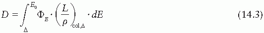

The use of stopping powers in photon and electron dosimetry has been discussed in Chapter 8. Quantitative data on stopping powers as a function of electron energy for various elements and materials have been calculated by Berger and Seltzer (9,10) and tabulated in Table A.8 of the appendix. More extensive tables of stopping powers are given by the ICRU (11). National Institute of Standards and Technology (NIST) maintains a list of stopping powers calculated by Berger et al. (12) (http://physics.nist.gov/PhysRefData/Star/Text/ESTAR.html).


B. ELECTRON SCATTERING

When a beam of electrons passes through a medium, the electrons suffer multiple scattering due to Coulomb force interactions between the incident electrons and, predominantly, the nuclei of the medium. As a result, the electrons acquire velocity components and displacements transverse to their original direction of motion. For most practical applications, the angular and spatial spread of a narrow, collimated beam of electrons can be approximated by a Gaussian distribution (13).

By analogy with mass stopping power, the ICRU (8) defines the mass angular scattering power of the material as the quotient, image, where image 
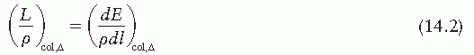
is the mean square scattering angle. Following the calculations of Rossi (13), mass scattering powers for various materials and electron energies have been tabulated (14).

The scattering power varies approximately as the square of the atomic number and inversely as the square of the kinetic energy. For this reason, high-Z materials are used in the construction of scattering foils. Scattering foils spread out the electron beam that emerges from the accelerator tube, and are made thin to minimize x-ray contamination of the electron beam.


14.2. ENERGY SPECIFICATION AND MEASUREMENT

Although an electron beam is almost monoenergetic before exiting the accelerator structure, the random energy degradation that the electrons suffer as they pass through the exit window, scattering foil, monitor chambers, air, and other materials results in the beam taking on a spectrum of energies at the phantom surface. Further degradation and spread of beam energy take place with depth in the phantom (Fig. 14.2).

In clinical practice, an electron beam is usually characterized by the energy at the body surface. There are several methods that can be used to determine this energy: measurement of
threshold energy for nuclear reactions; range measurements; and the measurement of Cerenkov radiation threshold (14). Of these, the range method is the most practical and convenient for clinical use.


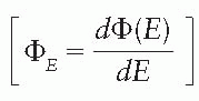
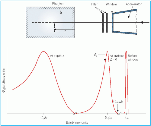
Figure 14.2. Distribution of electron fluence in energy, øE, as the beam passes through the collimation system of the accelerator and the phantom. (From International Commission on Radiation Units and Measurements. Radiation Dosimetry: Electrons with Initial Energies between 1 and 50 MeV. Report No. 21. Washington, DC: International Commission on Radiation Units and Measurements; 1972, with permission.)


A. MOST PROBABLE ENERGY

The Nordic Association of Clinical Physics (15) recommends the specification of most probable energy, (Ep)0 (defined by the position of the spectral peak in Fig. 14.2) at the phantom surface and the use of the following relationship:


where Rp is the practical range in centimeters as defined in Figure 14.3. For water, C1 = 0.22 MeV, C2 = 1.98 MeV/cm, and C3 = 0.0025 MeV/cm2 (16, 17, 18). They further recommend that the field size for range measurements be no less than 12 × 12 cm2 for energies up to 10 MeV and no less than 20 × 20 cm2 for higher energies.

For the determination of range, ion chambers, diodes, or film may be used. Although the range measurements are usually made using the depth ionization curve, the result is only slightly different from what would be obtained using depth dose curves (19). The practical range, Rp, is the depth of the point where the tangent to the descending linear portion of the curve (at the point of inflection) intersects the extrapolated background, as shown in Figure 14.3.

To be in strict accordance with Equation 14.4, each point on the depth ionization curve should be corrected for beam divergence before the range is determined. The correction factor is image
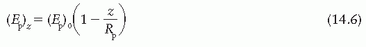
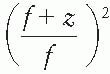
, where f is the effective source to surface distance (SSD); see Section 14.4E for details) and z is the depth. However, this correction in Rp is clinically not significant in terms of its impact on the ionization to dose conversion factor (20).


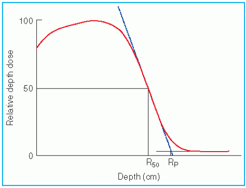
Figure 14.3. Depth dose curve illustrating the definition of Rp and R50.


B. MEAN ENERGY

It has been shown (21) that the mean energy of the electron beam, Ē0, at the phantom surface is related to R50 (the depth at which the dose is 50% of the maximum dose) by the following relationship:


where C4 = 2.33 MeV/cm for water. Again, the divergence correction is applied to each point on the depth dose curve before determining R50.

The American Association of Physicists in Medicine (AAPM) TG-21 protocol recommended the value of C4 as 2.33 MeV/cm. However, Monte Carlo calculations of Rogers and Bielajew (22) have shown that the value of C4 in the energy range of clinical interest is closer to 2.4 MeV/cm. Again, this small change in the value of C4 as well as the divergence correction mentioned above has little impact on clinical dosimetry (20).


C. ENERGY AT DEPTH

Harder (23) has shown that the most probable energy and, approximately, the mean energy of the spectrum decrease linearly with depth. This can be expressed by the relationships:


and approximately


where z is the depth.

Equation 14.7 is important in dosimetry because for absorbed dose measurements it is necessary to know the mean electron energy at the location of the chamber.


14.3. DETERMINATION OF ABSORBED DOSE

Calorimetry is the most basic method for the determination of absorbed dose, but because of technical difficulties, the use of calorimeters is not practical in a clinical setting. Ionization chambers and Fricke dosimeters are more commonly used. Film, thermoluminescent dosimeters (TLDs), and solid state diodes are used to find the ratio of the dose at one point in a phantom to the dose at another point but not usually to measure the absolute absorbed dose at a point.

Ionization chambers should be calibrated by an Accredited Dose Calibration Laboratory (ADCL) or the NIST. However, an ADCL can usually provide calibrations only for high-energy photon beams (60Co or 2-MV x-rays) but not for high-energy electron beams. The use of ionization chambers calibrated for photon beams for the measurement of absorbed dose in electron beams has been the subject of many national and international protocols (14,15,24, 25, 26). The most current recommendations are included in the protocols by TG-51 of the AAPM (24) and the International Atomic Energy Agency (IAEA) TRS398 (25). Elements of these protocols and other related concepts were presented in Chapter 8.


A. OUTPUT CALIBRATION

The variation of output (absorbed dose per monitor unit at dmax in phantom) with field size differs considerably from one type of accelerator to another. Therefore, the output of each treatment applicator or representative field size should be measured for each available energy. The output for one applicator or field size (often the 10 × 10-cm field) is selected as the standard to which the other output measurements are referred. Since the beam is calibrated to give 1 cGy/MU for the standard applicator at the depth of maximum dose on the central axis (nominal SSD = 100 cm), the output factor for any applicator represents cGy/MU at dmax. This topic will be further discussed in Section 14.4D.


B. DEPTH DOSE DISTRIBUTION

The depth dose and isodose distributions can be determined by ion chambers, diodes, or films. Automatic beam scanning systems and densitometers are useful in this regard and are available commercially.


B.1. Ionization Chambers

Although plane-parallel chambers are best suited for relative dose measurements in electron beams, cylindrical ionization chambers are also commonly used for the measurement of depth dose distribution. Depth ionization curves measured with an ion chamber need to be converted to depth dose curves by making the following corrections: (a) correction for restricted mass stopping power ratio of water to air, image, as a function of mean electron energy at depth; and (b) chamber replacement correction, Prepl. This factor is dependent both on the air cavity diameter as well as well as the mean electron energy at the depth of measurement.

Data for image are provided in the Appendix (Table A.3) as a function of incident electron beam energy and depth. The factor Prepl accounts for three effects: (a) the in-scatter effect, which increases the electron fluence in the chamber cavity because of electron scattering out of the air cavity being less than that expected in the intact medium; (b) the obliquity effect, which decreases the fluence in the cavity because of electrons travelling relatively straight in the air cavity instead of taking oblique paths as they would without cavity owing to larger-angle scattering in the medium than air; and (c) the displacement in the effective point of measurement. The first two effects may be grouped into a fluence correction, while the third is called the gradient correction.

Although the gradient correction for electrons is depth dependent, a single correction may be applied as an approximation to the entire depth ionization curve by shifting the curve toward the surface through a distance of 0.5r, where r is the radius of the chamber cavity (Chapter 8). The fluence correction is dependent on the chamber cavity radius as well as on the mean electron energy at depth, Ēz. Table 14.1 gives fluence correction factors for cylindrical chambers of different inner diameters as a function of mean energy at depth.

The following equation for the conversion of percent depth ionization, %DIw, in water to percent depth dose (PDD), %DDw, in water takes into account the above corrections:


The software for converting depth ionization curves to depth dose curves for electron beams may be available with the water phantom scanning systems.


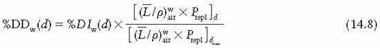
TABLE 14.1 Effective Density for Scaling Depth in Nonwater Phantoms to Water for Electron Beamsa


Material


Mass Density (g/cm3)


Effective Density Relative to Water


Water


1


1


Polystyrene (clear)


1.045


0.975


Polystyrene (high impact, white)


1.055


0.99


Acrylic


1.18


1.15


Electron solid water


1.04


1.00


aRecommended in American Association of Physicists in Medicine (AAPM). Clinical electron-beam dosimetry. AAPM Task Group No. 25. Med Phys. 1991;18:73.


It should be mentioned that for well-designed plane-parallel chambers with adequate guard rings, both the fluence and gradient corrections may be ignored (i.e., Prepl ≈ 1); the point of measurement for these chambers is defined at the front surface of the air cavity. However, image correction as a function of depth still needs to be applied.


B.2. Silicon Diodes

Silicon p-n junction diodes offer some advantages in terms of small size and high sensitivity (Chapter 8). However, diodes suffer from temperature and directional dependence and their sensitivity may change over time. Therefore, they are not recommended for absolute dosimetry. They are suitable for relative electron beam dosimetry such as measuring depth dose distribution. Because variation of silicon-to-water stopping power ratio with electron energy is quite minimal (˜5% between 1 and 20 MeV), measurements made with a diode may be used directly to give depth dose distributions. However, diode measurements should be checked by ion chamber measurements in order to ensure that the diode is functioning properly. Figure 14.4 shows a comparison of depth dose distributions obtained with an ion chamber (corrected for stopping power ratios and other effects) and a diode. The data show close agreement.


B.3. Film

Film dosimetry offers a convenient and rapid method of obtaining a complete set of isodose curves in the plane of the film. Its use for determining electron beam dose distributions is well established (27, 28, 29). It has been shown that the depth dose distributions measured by using film agree well with those by ion chambers when the latter measurements are corrected as outlined in Section 14.3B.1 (Fig. 14.5). Good agreement has also been demonstrated between film and FeSO4 dosimeters used for the measurement of depth dose curves (29). The energy independence of film may be explained by the fact that the ratio of collision stopping power in emulsion and in water varies slowly with electron energy (9). Thus, the optical density of the film can be taken as proportional to the dose with essentially no corrections.

Film is useful for a variety of dosimetry problems such as determining practical range, isodose curves, and beam flatness. However, film cannot be used reliably for absolute dosimetry because the optical density of a film exposed to electrons depends on many variables such as emulsion, processing conditions, magnitude of absorbed dose, and some measurement conditions, which can give rise to serious artifacts. The use of film is, therefore, restricted to
relative dosimetry. Care is required to avoid air gaps adjacent to the film. In addition, the sensitometric curve (optical density as a function of absorbed dose) must be known to interpret the optical density in terms of absorbed dose. Wherever possible, a film with a linear response over the range of measured dose should be used. Errors caused by changes in the processing conditions can be minimized by developing the films at approximately the same time. Accuracy can also be improved by using films from the same batch.


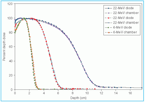
Figure 14.4. Comparison of depth dose curves measured with a diode and an ion chamber. Whereas the diode response was uncorrected, the chamber readings were corrected for change in image as a function of depth, and the displacement of the effective point of measurement. (From Khan FM. Clinical electron beam dosimetry. In: Keriakes JG, Elson HR, Born CG, eds. Radiation Oncology Physics—1986. AAPM Monograph No. 15. New York, NY: American Institute of Physics; 1986:211, with permission.)


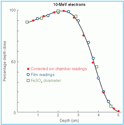
Figure 14.5. Comparison of central axis depth dose curve measured with an ion chamber, film, and FeSO4 dosimeter. (From Almond PR. Calibration of megavoltage electron radiotherapy beams. In: Waggener RG, Kereiakes JG, Shalek RJ, eds. Handbook of Medical Physics, Vol 1. Boca Raton, FL: CRC Press; 1982:173, with permission.)

Film can be positioned either perpendicular or parallel to the beam axis. In the latter case, precautions must be taken to align the top edge of the film with the surface of the phantom or serious artifacts and errors in the depth dose distribution may result (28) (Fig. 14.6).

To obtain isodose curves, the film is usually placed in a plastic phantom such as polystyrene or solid water and oriented parallel to the beam axis. The film can be kept in its original paper jacket and pressed tightly between the phantom slabs. Small holes can be punched in the corners of the jacket for trapped air to escape. The film wrapping that extends beyond the phantom should be folded to one side and taped down. After processing, the film may be analyzed using a densitometer having a light aperture of about 1 mm diameter. Figure 14.7 shows an example of a film exposed to electrons and a set of isodose curves obtained by isodensity scanning. Because the effective density of transparent polystyrene or solid water is close to that of water, the resulting isodose curves can be used clinically without further correction.

Because many electron energies are often available with accelerators, an automatic film dosimetry system is a desirable thing to have in a clinical department. Automatic density plotters are commercially available, and some of them are interfaced with treatment-planning computers. Although hand processing of films gives the best results, automatic rapid processors can be used in many instances. A strict quality assurance, however, is necessary to maintain consistency in film dosimetry.


B.4. Phantoms

Water is the standard phantom for the dosimetry of electron beams. However, it is not always possible or practical to perform dosimetry in a water phantom. For example, plastic phantoms are more suitable when using film or plane-parallel chambers. It also is difficult to make measurements near the surface of water, because of its surface tension and the uncertainty in positioning the detector near the surface.

For a phantom to be water equivalent for electron dosimetry it must have the same linear stopping power and the same linear angular scattering power. This is approximately achieved if the phantom has the same electron density (number of electrons per cubic centimeter) and the same effective atomic number as water. A depth dose distribution measured in a nonwater phantom may be converted to that expected in a water phantom by the following relationship (20):


provided the energy spectra of electrons at each position are identical. However, because of differences in stopping power and scattering power among different phantoms, it is not possible to find corresponding depths at which the energy spectra are identical. Consequently, there is no single scaling factor that can accurately transform an entire depth dose curve in a nonwater phantom to that in water. However, an effective density may be assigned to a medium to give water-equivalent depth dose distribution near the therapeutic range and along the descending portion of the depth dose curve. The AAPM (20) has recommended that the water-equivalent depth or the effective density (ρeff) may be estimated from the following relationship:


where R50 is the depth of 50% dose or detector response. Recommended values of ρeff for various phantoms are given in Table 14.1.


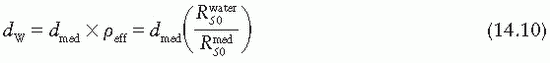
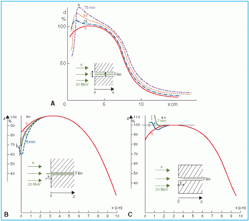
Figure 14.6. Film artifacts created by misalignment of the film in the phantom. The effects of A: air gaps between the film and the phantom, B: film edge extending beyond the phantom, and C: film edge recessed within the phantom. (From Dutreix J, Dutreix A. Film dosimetry of high energy electrons. Ann NY Acad Sci. 1969;161:33, with permission.)


14.4. CHARACTERISTICS OF CLINICAL ELECTRON BEAMS


A. CENTRAL AXIS DEPTH DOSE

The major attraction of the electron beam irradiation is the shape of the depth dose curve, especially in the energy range of 6 to 15 MeV. A region of more or less uniform dose followed by a rapid dropoff of dose offers a distinct clinical advantage over the conventional x-ray modalities. This dose gradient, however, decreases with increasing energy.

It was stated earlier that high-energy electrons lose energy at the rate of about 2 MeV/cm of water or soft tissue. Beyond the maximum range of electrons, the dose is contributed only by the x-ray contamination of the beam, indicated by the tail of the depth dose curve (Fig. 14.8).


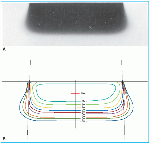
Figure 14.7. Film used for obtaining isodose curves. A: A film exposed to 12-MeV electron beam, 14 × 8-cm cone, in a polystyrene phantom. B: Isodensity curves.


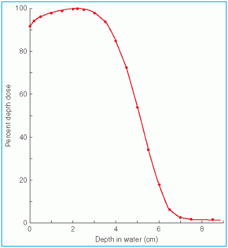
Figure 14.8. Central axis depth dose distribution measured in water. Incident energy (Ep)0 = 13 MeV; 8 × 10-cm cone; effective source to surface distance = 68 cm.


For a broad beam, the depth in centimeters at which electrons deliver a dose to the 80% to 90% isodose level is equal to approximately one-third to one-fourth of the electron energy in MeV. Thus, a 13-MeV electron beam is useful to a depth of about 3 to 4 cm, depending on the isodose level specified. As seen in Figure 14.8, the depth dose curve falls off sharply beyond the useful depth and, therefore, the underlying tissues are spared.

The most useful treatment depth, or therapeutic range, of electrons is given by the depth of the 90% depth dose. For modern accelerators with trimmer-type applicators this depth is approximately given by E/3.2 cm, where E is the most probable energy in MeV of the electron beam at the surface. The depth of the 80% depth dose occurs approximately at E/2.8 cm. The depth of Dmax does not follow a linear relationship with energy but it covers a broad region and its value may be approximated by 0.46 E0.67 (30). Figure 14.9 shows a comparison of depth of 90% dose (R90) as a function of beam energy for two different linear accelerators. These differences can be clinically significant and, therefore, underscore the requirement of using beam data that have been measured specifically for the given machine.


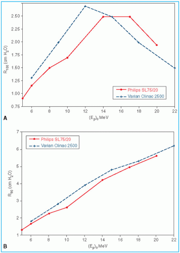
Figure 14.9. Plots of depth dose ranges as a function of the most probable energy (Ep)0 at the surface for two different linear accelerators. A: R100, the depth of maximum dose versus (Ep)0. B: R90, the depth of 90% depth dose versus (Ep)0. (From Khan FM. Clinical electron beam dosimetry. In: Keriakes JG, Elson HR, Born CG, eds. Radiation Oncology Physics—1986. AAPM Monograph No. 15. New York, NY: American Institute of Physics; 1986:211, with permission.)


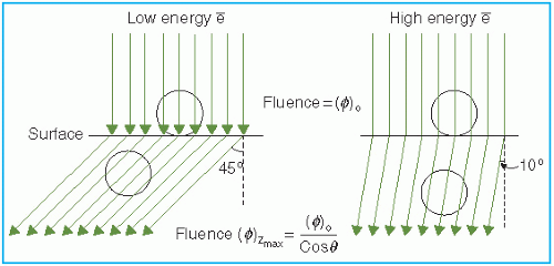
Figure 14.10. Schematic illustration showing the increase in percent surface dose with an increase in electron energy. (From Khan FM. Clinical electron beam dosimetry. In: Keriakes JG, Elson HR, Born CG, eds. Radiation Oncology Physics—1986. AAPM Monograph No. 15. New York, NY: American Institute of Physics; 1986:211, with permission.)


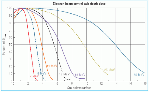
Figure 14.11. Comparison of central axis depth dose distributions of the Sagittaire linear accelerator (continuous curves) and the Siemen’s betatron (dashed curves). (From Tapley N, ed. Clinical Applications of the Electron Beam. New York, NY: John Wiley & Sons; 1976, with permission.)

The choice of beam energy is much more critical for electrons than for photons. Because the dose decreases abruptly beyond the 90% dose level, the treatment depth and the required electron energy must be chosen very carefully. The guiding principle is that, when in doubt, use higher electron energy to make sure that the target volume is well within the specified isodose curve.

The skin-sparing effect with the clinical electron beams is only modest or nonexistent. Unlike the photon beams, the percent surface dose for electrons increases with energy. This effect can be explained by the nature of the electron scatter. At the lower energies, the electrons are scattered more easily and through larger angles. This causes the dose to build up more rapidly and over a shorter distance. The ratio of surface dose to maximum dose is, therefore, less for the lower-energy electrons than for the higher-energy electrons. A simple illustration of this effect is seen in Figure 14.10. For the same incident electron fluence (e/cm2), the lower-energy electrons build up to a larger fluence at the depth of maximum dose than the higher-energy electrons. The increase in fluence is given by 1/cos θ, where θ is the angle of scatter.

Because of differences in beam generation, beam bending, and collimation, the depth dose distribution and the surface dose can be significantly different for different machines. Figure 14.11 illustrates this point by comparing central axis depth dose curves for the Sagittaire linear accelerator and the Siemen betatron for different beam energies. In clinical practice, therefore, it is not sufficient to specify just beam energy. Isodose distributions for an individual machine, cone, and/or field size are required.


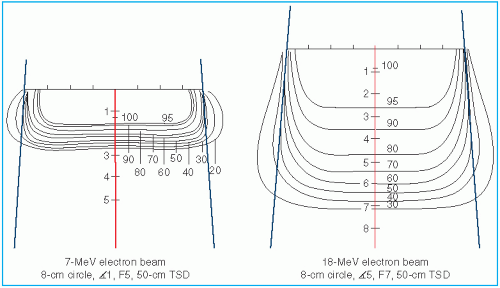
Figure 14.12. Comparison of isodose curves for different energy electron beams. (From Tapley N, ed. Clinical Applications of the Electron Beam. New York, NY: John Wiley & Sons; 1976:86, with permission.)


B. ISODOSE CURVES

The scattering of electrons plays an important role in determining the shape of the isodose curves— the central axis distribution, flatness, and curvature near the field borders. Significant differences exist among the shapes of the isodose curves for different machines. These differences arise as a result of different collimation systems that the accelerators employ. The collimation system (e.g., scattering foil, monitor chambers, jaws, and cones) and the air column above the patient cause an angular dispersion of the beam as well as energy spread. Thus, two beams of the same energy, E0, can give rise to different dose distributions after passing through different collimation systems.

As the beam penetrates a medium, the beam expands rapidly below the surface due to scattering. However, individual spread of the isodose curves varies, depending on the isodose level, energy, field size, and collimation. Figure 14.12 shows isodose patterns for two different energy beams. Whereas for the low-energy beams all the isodose curves show some expansion, for the higher energies only the low-value isodose levels bulge out. The higher isodose levels tend to show lateral constriction, which becomes worse with decreasing field size.


C. FIELD FLATNESS AND SYMMETRY

Uniformity of the electron beam is usually specified in a plane perpendicular to the beam axis and at a fixed depth. The ICRU (31) specifies beam flatness in terms of a uniformity index. This is defined in a reference plane and at a reference depth as the ratio of the area where the dose exceeds 90% of its value at the central axis to the geometric beam cross-sectional area at the phantom surface. The uniformity index should exceed a given fraction (e.g., 0.80 for a 10 × 10-cm field size and at depth of maximum dose). In addition, the dose at any arbitrary point in the reference plane should not exceed 103% of the central axis value.

Figure 14.13 shows isodose curves obtained from a film exposed perpendicular to an electron beam at the depth of maximum dose. The dashed line is the boundary of the geometric beam at the surface. In this example, the homogeneity index is 0.8.

Because of the presence of lower-energy electrons in the beam, the flatness changes significantly with depth. Therefore, it has been recommended (32) that the uniformity index be defined at the depth of half the therapeutic range (e.g., one-half the depth of 85% depth dose). Furthermore, it is defined as the ratio of the areas inside the 90% and 50% isodose lines at this depth. A uniformity index of 0.70 or higher is acceptable with field sizes larger than 100 cm2. The peak value in this plane should be less than 103%.

The AAPM (20) recommends that the flatness of an electron beam be specified in a reference plane perpendicular to the central axis, at the depth of the 95% isodose beyond the depth of dose maximum. The variation in dose relative to the dose at central axis should not exceed ±5% (optimally to be within ±3%) over an area confined within lines 2 cm inside the geometric edge of fields equal to or larger than 10 × 10 cm2.


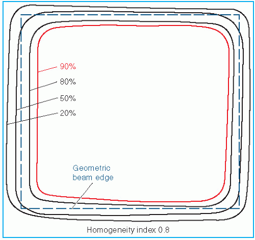
Figure 14.13. Isodose curves in a plane perpendicular to the central axis, obtained with a film placed in a phantom at the depth of maximum dose. (From Almond PR. Radiation physics of electron beams. In: Tapley N, ed. Clinical Applications of the Electron Beam. New York, NY: John Wiley & Sons; 1976:50, with permission.)

Beam symmetry compares a lateral dose profile on one side of the central axis to that on the other. The AAPM recommends that the cross-beam profile in the reference plane should not differ more than 2% at any pair of points located symmetrically on opposite sides of the central axis.


C.1. Beam Collimation

Acceptable field flatness and symmetry are obtained with a proper design of beam scatterers and beam-defining collimators. Accelerators with magnetically scanned beam do not require scattering foils. Others use one or more scattering foils, usually made up of lead, to widen the beam as well as give a uniform dose distribution across the treatment field.

The beam collimation has been significantly improved by the introduction of the dual-foil system (33). Figure 14.14 shows a typical arrangement for such a system. Whereas the first foil widens the beam by multiple scattering, the second foil is designed to make the beam uniform in cross section. The thickness of the second foil is differentially varied across the beam to produce
a desired degree of beam widening and flattening. Analysis by Werner et al. (34) shows that the dual-foil systems compare well with the scanning beam systems in minimizing angular spread and, hence, the effect on dose distribution characteristics.


Figure 14.14. Principle of dual-foil system for obtaining uniform electron beam field. (From Almond PR. Handbook of Medical Physics. Vol I. Boca Raton, FL: CRC Press; 1982:149, with permission.)

The beam-defining collimators are designed to provide a variety of field sizes and to maintain or improve the flatness of the beam. Basically, all collimators provide a primary collimation close to the source that defines the maximum field size and a secondary collimation close to the patient to define the treatment field. The latter can be in the form of trimmer bars or a series of different applicators. In the electron therapy mode, the x-ray collimator jaws are usually opened to a size larger than the applicator opening. Because the x-ray jaws give rise to extensive electron scatter, they are interlocked with the individual applicators to open automatically to a fixed predetermined size.


D. FIELD SIZE DEPENDENCE

The output and the central axis depth dose distribution are field size dependent. The dose increases with field size because of the increased scatter from the collimator and the phantom. As stated previously, some electron collimators provide a fixed jaw opening, and the treatment field size is varied by various-size applicators (also called cones), inserts, or movable trimmer bars. Such an arrangement minimizes the variation of collimator scatter, and therefore, the output variation with field size is kept reasonably small. If the collimator aperture (x-ray jaw setting) were allowed to change with the treatment field, the output would vary too widely with field size, especially for lower-energy beams. This effect is shown in Figure 14.15, where the applicator size is held fixed, while the x-ray jaws are varied (35). Note that the dose rate varies by a factor of greater than 2 between small and large jaw openings at 4 MeV.

The effects of field size on output and the central axis depth dose curve due to phantom scatter is significant as long as the distance between the point of measurement and the edge of the field is shorter than the range of the laterally scattered electrons. After this distance is reached, there is no further increase in depth dose caused by phantom scatter. When the field size is reduced below that required for lateral scatter equilibrium (LSE), the dose rate decreases rapidly. This is shown in Figure 14.16. In these measurements, the field size at the phantom was varied without changing the photon collimator opening. For small fields, the output factor as well as depth dose can be significantly reduced compared with the broad beam distribution.

Figure 14.17 shows the change in central axis depth dose distribution with field size. As the field size is increased, the PDD initially increases but becomes constant beyond a certain field size when the LSE is reached. Furthermore, the depth dmax shifts toward the surface for the smaller fields. Thus, in clinical practice, depth dose distribution for small fields should be measured individually in addition to the output calibration.


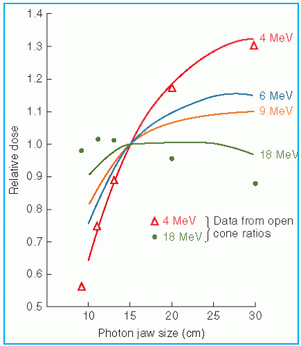
Figure 14.15. Variation of relative dose at dmax, through a 10 × 10-cm cone, with change of jaw setting, relative to the recommended jaw setting. (From Biggs PJ, Boyer AL, Doppke KP. Electron dosimetry of irregular fields on the Clinac-18. Int J Radiat Oncol Biol Phys. 1979;5:433, with permission.)


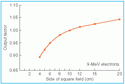
Figure 14.16. Output factors as a function of side of the square field. Primary collimator fixed, secondary collimators (trimmers) close to the phantom varied to change the field size. Data are from Therac 20 linear accelerator. (From Mills MD, Hogstrom KR, Almond PR. Prediction of electron beam output factors. Med Phys. 1982;9:60, with permission.)

It has been shown (36) that the minimum field radius for the establishment of LSE at all depths on central axis is given by the following approximate relationship:


where Req is the field radius in cm and Ep,o is the most probable energy at the surface in MeV. For example, the equilibrium fields for 8- and 32-MeV electrons have diameters of 5 and 10 cm, respectively, which agree with the data shown in Figure 14.17. In clinical practice, the above relationship may be used to classify fields with radius less than Req as small or narrow fields and radius greater than or equal to Req as broad fields. Thus, as stated earlier, the depth dose distribution for small fields is field size dependent, while for broad fields it is independent of field size.


E. FIELD EQUIVALENCE

Exact field equivalence for electron beams of different shapes cannot be established. However, it has been shown (36) that approximate equivalent circular or square fields can be determined for fields of any size, shape, and energy. The term field equivalence means that for the same
incident fluence and cross-sectional beam uniformity, the equivalent fields have the same depth dose distribution along the central ray. Thus, field equivalence here is defined in terms of PDDs and not the output factors, which depend on particular jaw setting for the given applicator or other collimation conditions. According to this definition, all broad fields are equivalent because their depth dose distribution is the same irrespective of field size. For example, 10 × 10, 10 × 15, 10 × 20, and 20 × 20 are all broad fields for energies up to 30 MeV (see Equation 14.11) and hence are equivalent in depth dose distribution. Field equivalence is therefore relevant only for small fields in which the LSE does not exist, and consequently, the depth dose distribution is field size dependent.


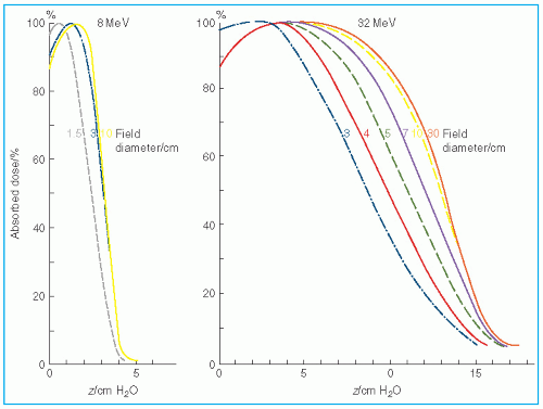
Figure 14.17. Variation of depth dose distribution with field size. (From International Commission on Radiation Units and Measurements. Radiation Dosimetry: Electron Beams with Energies between 1 and 50 MeV. Report No. 35. Bethesda, MD: International Commission on Radiation Units and Measurements; 1984, with permission.)

Harder et al. (37) have shown that for a square field of dimensions (a × a), the equivalent circular field has a diameter Dequiv, given by


However, for small rectangular or irregularly shaped fields, field equivalence is not as straightforward. Khan and Higgins (36) have applied Gaussian pencil beam theory to this problem and derived relationships that can be used to find approximate equivalent circular or square fields for fields of any size and shape. The reader is referred to their paper for further details on this subject.


F. SQUARE ROOT METHOD

Hogstrom et al. (38) have shown that, if the change in collimator scatter with field size is not considered, the depth dose for rectangular field sizes can be extracted from square field data by the following relationship:


where D is the central axis depth dose and X and Y are the field dimensions. Thus, the depth dose for a rectangular field size can be determined from the square root of the two square field depth doses when the sides of the two square fields are equal respectively to the two sides of the rectangular field.

Referred to as the square root method, this concept has also been applied to the determination of output factors when the primary collimation is fixed and the secondary collimation close to the phantom is varied (39). It may be restated that the collimator scatter is neglected in this model. Thus, the applicability of the square root method is not automatically valid for those machines in which collimator scatter varies significantly with field size.


G. ELECTRON SOURCE

Unlike an x-ray beam, an electron beam does not emanate from a physical source in the accelerator head. A pencil electron beam, after passing through the vacuum window of the accelerator, bending magnetic field, scattering foils, monitor chambers, and the intervening air column, is spread into a broader beam that appears to diverge from a point. This point is called the virtual source (40), which may be defined as an intersection point of the backprojections along the most probable directions of electron motion at the patient surface (41). This is illustrated in Figure 14.18.

A number of methods have been suggested for the determination of virtual source position. Pohlit’s (40) method consists of taking electron radiographs of a grid of copper wires at different distances from the collimator and backprojecting the images to a point, the virtual source. A multipinhole technique (41) uses double conical holes in a metal plate. Pinhole images are obtained on a film. Backprojection of the pinhole images gives the virtual source position. Meyer et al. (42) have described the method of determining field size magnification on film with distance. The virtual source point is found by the backprojection of the 50% width of the beam profiles obtained at different distances. A broad beam (≥20 × 20 cm2) is used for these measurements.

The use of virtual SSD does not give accurate inverse square law correction for output at extended SSDs under all clinical conditions. Measurements have shown that the virtual SSD gives correct inverse square law factor only for large field sizes (43). For small field sizes, the inverse square law correction underestimates the change in output with virtual SSD. This deviation from the inverse square law is caused by an additional decrease in output because of a loss of side-scatter equilibrium in air and in phantom that is significant for small field sizes and low electron energies. Thus, the use of the virtual SSD to predict dose variation with distance requires correction factors, in addition to the inverse square law factor, as a function of field size and energy (42).

An alternative method of correcting dose output as a function of air gap between the electron applicator end and the patient is to determine a quantity known as the effective SSD. The
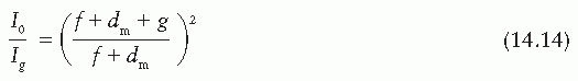
effective SSD is defined as the distance from an effective source position to the standard phantom position (e.g., isocenter) which gives the correct inverse square law relationship for the change in output with distance. Khan et al. (44) have recommended a method that simulates as closely as possible the clinical situation. In this method, doses are measured in a phantom at the depth of maximum dose (dm), with the phantom first at the standard SSD (zero gap) and then at various distances, up to about 20 cm from the applicator end. Suppose f = effective SSD, I0 = dose with zero gap, and Ig = dose with gap g between the standard SSD point and the phantom surface. Then, if electrons obey inverse square law,


or


By plotting image 
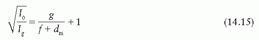
as a function of gap g (Fig. 14.19), a straight line is obtained, the slope of which is image. Thus the effective SSD is given by
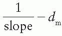
 image.


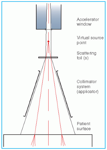
Figure 14.18. Definition of the virtual point source of an electron beam: the intersection point of the backprojections along the most probable directions of motion of electrons at the patient surface. (From Schroeder-Babo P. Determination of the virtual electron source of a betatron. Acta Radiol. 1983;364(suppl):7, with permission.)

Although the effective SSD is obtained by making measurements at the depth dm, its value does not change significantly with the depth of measurement (44). However, the effective SSD does change with energy and field size, especially for small field sizes and low energies. A table of effective SSDs as a function of energy and field size may be made available as part of the beam data to meet clinical situations.


H. X-RAY CONTAMINATION

Dose due to x-ray contamination at the end of the electron range can be determined from the tail of the depth dose curve by reading off the dose value at the point where the tail becomes straight (Fig. 14.3). This dose in a patient is contributed by bremsstrahlung interactions of electrons with the collimation system (scattering foils, chambers, collimator jaws, etc.) and the body tissues. Table 14.2 gives the x-ray dose generated in water for monoenergetic electron beams, with no initial x-ray contamination. These values were extracted from the depth dose distributions in water calculated by Berger and Seltzer (45), using a Monte Carlo program. The x-ray contamination dose from a medical accelerator, however, depends very much on its collimation system and is usually an order of two greater than the values given in Table 14.2. In general, the x-ray contamination is least in the scanning beam type of accelerator, because the
scattering foils are not used. In a modern linear accelerator, typical x-ray contamination dose to a patient ranges from approximately 0.5% to 1% in the energy range of 6 to 12 MeV; 1% to 2%, from 12 to 15 MeV; and 2% to 5%, from 15 to 20 MeV.


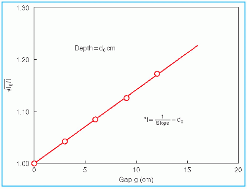
Figure 14.19. Determination of the effective source to surface distance. (From Khan FM, Sewchand W, Levitt SH. Effect of air space on depth dose in electron beam therapy. Radiology. 1978;126:249, with permission.)


TABLE 14.2 X-ray Contamination Dose (Dx) to Water, at the End of the Electron Range as a Percentage of Dmax


Energy (MeV)


Dx (%)


5


0.1


10


0.5


15


0.9


20


1.4


30


2.8


40


4.2


50


6.0


(Data are for theoretical beam with no initial x-ray contamination and are extracted from Monte Carlo data of Berger MJ, Seltzer SM. Tables of Energy-Deposition Distributions in Water Phantoms Irradiated by Point-Monodirectional Electron Beams with Energies from 1 to 60 MeV, and Applications to Broad Beams. NBSIR 82-2451. Washington, DC: National Bureau of Standards; 1982.)


For regular treatment field sizes used in electron beam therapy, the dose to the patient contributed by the x-ray contamination is not of much concern. However, even small amounts of x-ray contamination become critical for total skin electron irradiation such as in the treatment of mycosis fungoides (Section 14.8).


14.5. TREATMENT PLANNING

Most electron beam treatments are planned for a single field technique. For a relatively flat and homogeneous slab of soft tissue, the dose distribution can be found by using the appropriate isodose chart. However, this simplicity of treatment planning is the exception rather than the rule. Surface areas are seldom flat, and in many cases, inhomogeneities, such as bone, lung, and air cavities, present dosimetric complexities.

Before the advent of computer treatment planning for electron beams, planning methods were rudimentary and involved manual techniques of modifying standard isodose charts measured in a water phantom. Empirically determined correction factors were applied to correct dose

Only gold members can continue reading. Log In or Register to continue

Stay updated, free articles. Join our Telegram channel

Jun 8, 2016 | Posted by in GENERAL RADIOLOGY | Comments Off on Electron Beam Therapy

Full access? Get Clinical Tree

Get Clinical Tree app for offline access