Fast Spin Echo
Introduction
In this chapter, we will discuss the elegant and cunning technique of fast spin echo. This technique was first proposed by Hennig et al.1 and was called RARE (rapid acquisition with relaxation enhancement). However, it is commonly referred to as fast spin echo (FSE) or turbo spin echo (TSE). Different manufacturers have different names for it (Table 19-1).
Consider the pulse sequence diagram in Figure 19-1. This pulse sequence can be used for either a CSE or an FSE study.
Conventional Spin Echo
Let’s first talk about a conventional spin echo (CSE or SE) study and again see how the lines in k-space are filled in. With a CSE, immediately after the 90° RF pulse, an FID (free induction decay) is formed. At a time TE after the first 90° pulse (time TE/2 after the first 180° refocusing pulse—17 msec in our example), we receive the first spin echo. We have a whole train of 180° refocusing pulses, after each of which we get another echo. Each echo is a multiple of 17 msec. Notice that each successive echo has less amplitude as a result of T2 decay.
In a CSE sequence, we can get two echoes, that is, we apply two 180° RF pulses and get back an echo from each pulse, each with a different TE. However, we could have as many echoes as we want in a CSE sequence. In our example, we have an eight-echo sequence, all easily occurring within the time of one TR.
With each TR in a CSE, we have a single phase-encoding step. Each of the echoes following each 180° pulse is obtained after a single application of the phase-encoding gradient in CSE. Each echo has its own k-space, and each time we get an echo, we fill in one line of k-space (Fig. 19-1).
In CSE, each k-space will generate a different image, that is, we’ll get a first echo image, a second echo image, and so on. With eight 180° pulses generating eight echoes, we’ll have eight different k-spaces and eight different images. If we had 256 different phase-encoding steps, we would do this 256 different times. The scan time would be Scan time = (TR) (number of phase-encoding steps) (number of excitations [NEX]) Within the scan time, we’ll get eight images, one of each TE echo. If we were only interested in the last echo image, we wouldn’t have to bother with filling in the k-spaces for the first seven echoes. However, the first seven echoes come “free.” We don’t save any time by not doing them because we have to wait out the time it takes to
get to the last echo anyway. In a dual-echo CSE sequence, the first echo is always “free”—it doesn’t cost any time. (However, as we shall see later, that isn’t true with FSE.)
get to the last echo anyway. In a dual-echo CSE sequence, the first echo is always “free”—it doesn’t cost any time. (However, as we shall see later, that isn’t true with FSE.)
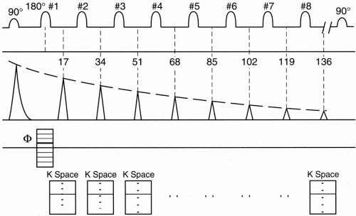
Thus, for each k-space in CSE, we repeat the TR 256 times (each at a different phase-encoding gradient) and fill in the k-space for each echo with 256 different lines. For an eight-echo train, we get eight different images.
Fast Spin Echo
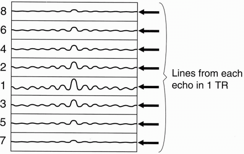
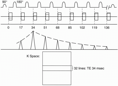
By using the same example, we can see how FSE works. FSE is a very elegant way of manipulating the CSE technique to save time. Again, we’ll start with a train of eight echoes (ETL = 8). However, now we will only have one k-space. We’ll fill this k-space eight lines at a time (Fig. 19-2). Instead of having eight separate
k-spaces, one for each echo, we will have one k-space using the data from all eight echoes.
k-spaces, one for each echo, we will have one k-space using the data from all eight echoes.
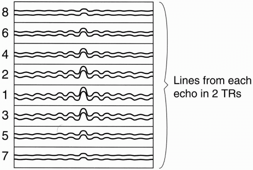 Figure 19-3. After two shots, 16 lines in k-space will be filled. |
Within the time of one TR (one “shot”), we will get eight lines, one from each echo, in the single k-space. With the next TR, we’ll accumulate eight more lines, one from each echo, and we’ll also put them into the same k-space (Fig. 19-3).
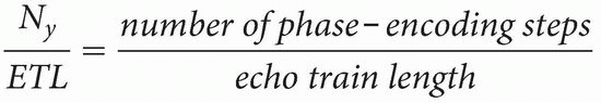
For each shot/TR, we will fill in another eight lines into the single k-space. Because we have a total of 256 lines in k-space, and because during each TR we are filling in eight lines of k-space at a shot, we only have to repeat the process 32 times (i.e., 256/8 = 32) to fill 256 lines of k-space.
In CSE, it took one TR for each line of k-space. Therefore, in a CSE study, we have to repeat the TR 256 times. In this manner, we have cut the time of the study by a factor of eight.
Echo Train Length
Echo train length (ETL) refers to the number of echoes used in FSE. The ETL ranges typically from 3 to 32. The time interval between successive echoes (or between 180° pulses) is called the echo spacing (ESP). A typical ESP is on the order of 16 to 20 msec at a typical high field bandwidth (BW) of 32 kHz (±16 kHz).
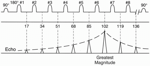
Figure 19-4 is an example. Let’s say we want an image with contrast reflecting a TE of approximately 100 msec. In FSE, the only TEs we can choose are integral multiples of the ESP (ESP = 17 msec in our example). This is called the effective TE (TEeff). We will see shortly that this is not a true TE. Therefore, in our example, TEeff=102 msec (= 6 × 17 msec).
Remember that the center of k-space has maximum signal, and as we go out to the edges of k-space, we get less and less signal. Therefore, if we divide k-space into 8 slabs of 32 lines each (1 slab for each echo), the center slab will be assigned to the sixth echo, that is, the echo corresponding to the chosen TEeff = 102 msec (Fig. 19-5).
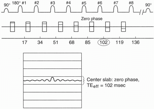 |
In FSE, before each 180° pulse, we place a different value of the phase-encoding gradient. For the 180° pulse before the echo we choose as the TEeff (in this case, 102 msec), we use a phaseencoding gradient with the lowest strength. Each subsequent phase-encoding step will have a gradient with more and more amplitude. This increase will result in the most signal coming from the echo at 102 msec (because this signal is obtained with a minimum phase gradient) and
decreasing signal from all the other echoes because their signals are obtained with increasing phase-encoding gradients (Fig. 19-6).
decreasing signal from all the other echoes because their signals are obtained with increasing phase-encoding gradients (Fig. 19-6).
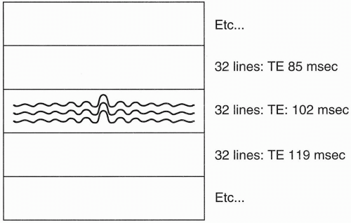 Figure 19-5. The 32 lines in the center of k-space correspond to the echoes associated with the weakest phase gradients. |
In the next TR, we again pick a phase-encoding step for the sixth echo that will be close to zero gradient and all the other phase-encoding steps will be close to their previous respective gradient values, so that again the maximum signal during this TR will be obtained from echo 6 (TE = 102 msec) and progressively weaker signals will be obtained from the other echoes.
The signals from the sixth echo (from the 1st to the 32nd TR) will all be placed in the center of k-space (Fig. 19-5). The signals from the other echoes will be placed in the other slabs. The echoes that experience progressively greater phase-encoding gradients (and therefore less signal) fall into slabs further away from the center slab, and those echoes experiencing the weakest phase-encoding gradients (and therefore having more signal) are placed closer to the center slab. k-space is organized so that the greatest amount of signal comes from the center of k-space and the least amount of signal comes from the periphery of k-space.
Therefore, if we choose an ETL of 8 echoes, we will have 8 slabs in k-space, with each slab containing 32 lines from 32 shots. Echo slab corresponds to a different echo. Let’s see what the echo looks like (Fig. 19-6).
Because the center slab belongs to the lowest phase-encoding gradient, it will have the least amount of dephasing. The signal received at TE =102 msec will have the greatest amplitude. As we go farther away from 102 msec in either direction, the signal amplitude will get progressively smaller because the phase-encoding gradients get progressively larger.
By definition, the maximum signal comes at the TEeff time. But we still get echoes from the other TEs that do not help our contrast. The signals from these other echoes are all in the same k-space. Even though the respective signal amplitudes from the other TEs are progressively smaller, the further away in time they are from the TEeff; they still contribute to the contrast from the TEeff. This is why it is called an effective TE and not a true TE.
In a way, what we are doing is averaging the echoes, although it is a weighted average. By appropriately picking the slabs, we put most of the weight on the echo corresponding to 102 msec (the TEeff) and less weight on the other echoes. As we go away from the center slab of k-space, we are reducing the weighting, that is, we are reducing the contribution of the data on that slab to the effective echo.
The previous example gives us a long TR/long TE, which is a T2-weighted image. Now we want to do a proton density-weighted image with a long TR/short TE and a TEeff of approximately 30 msec (Fig. 19-7). In this case, we would assign the center slab of k-space to correspond to the second echo, that is, TE =
34 msec. The echo with maximum magnitude will be at a TE of 34 msec, and the magnitude of the signal would fall off progressively with subsequent echoes. This is because, now, the second echo will be assigned the weakest phaseencoding gradients, and the subsequent echoes will have progressively stronger phase-encoding gradients.
34 msec. The echo with maximum magnitude will be at a TE of 34 msec, and the magnitude of the signal would fall off progressively with subsequent echoes. This is because, now, the second echo will be assigned the weakest phaseencoding gradients, and the subsequent echoes will have progressively stronger phase-encoding gradients.
 |
Remember that with the TEeff of 34 msec, we are still getting the cumulative signal from the entire echo train of eight echoes. So even information from an echo corresponding to a TE of 136 msec (8 × 17 = 136) is contributing to the signal of the TEeff of 34 msec, which we don’t want. Therefore, for a T1-weighted study, we usually pick a smaller ETL such as 4. With an ETL of 4, we would only do four phase-encoding steps. Thus, k-space would only have four slabs, and the longest echo contributing to the contrast of the shortest TEeff (e.g., 17 msec) would be the echo at 68 msec (4 × 17 = 68). This will eliminate the T2 effect on a T1-weighted image caused by the signal contribution of the longer echo times.
Question: What happens to the time it takes to do an FSE study when we decrease the ETL from 8 to 4?
Answer: The time of the study will be increased by a factor of 2.
Answer: We fill in eight lines of k-space with each TR, each line going to a separate slab within k-space.
Question: How many times do we have to repeat the TR to fill up k-space with 256 lines?
Answer: In general, we have to repeat it by the following ratio:
Remember that scan time is calculated by the following formula:
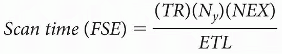
The numerator of the formula is the same as for a CSE study:
Scan time (CSE) = (TR


Related posts:
Stay updated, free articles. Join our Telegram channel
Full access? Get Clinical Tree
