Fourier Transform
Introduction
Fourier was an 18th century French mathematician. His picture, along with the Fourier transform of his picture, is shown in Figure 9-1. The Fourier transform (FT) is a mystery to most radiologists. Although the mathematics of FT is complex, its concept is easy to grasp. Basically, the FT provides a frequency spectrum of a signal. It is sometimes easier to work in the frequency domain and later convert back to the time domain.
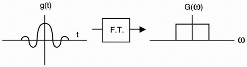
Let’s start by saying that we have a signal g(t), with a certain waveform (Fig. 9-2). This signal is basically a time function, that is, a waveform that varies with time. Now, let’s say we have a “black box” that converts the signal into its frequency components. The conversion that occurs in the “black box” is the Fourier transform. The FT converts the signal from the time domain to the frequency domain (Fig. 9-2). The FT of g(t) is denoted G(ω). (The frequency can be angular [ω] or linear [f].)
The FT is a mathematical equation (you don’t have to memorize it). It is shown here to demonstrate that a relationship exists between the signal in the time domain g(t) and its Fourier transform G(ω) in the frequency domain:
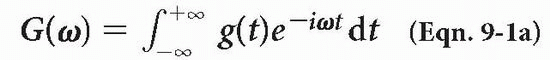
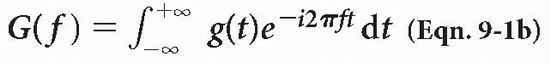
where ω = 2πf.
We are already familiar with the term (e−iωt) from Chapter 1. This is the term for a vector spinning with angular frequency ω. The formula integrates the product of this periodic function and g(t) with respect to time. It also provides another function, G(ω), in the frequency domain (Fig. 9-2).
One interesting thing about the Fourier transform is that the Fourier transform of the Fourier transform provides the original signal. If the Fourier transform of g(t) is G(ω), then the Fourier transform of G(ω) is g(t):

FT provides the range of frequencies that are in the signal. Here are some examples of functions and their Fourier transforms:
Example 1
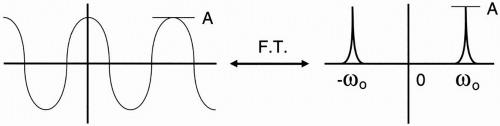
The cosine function: cos (ω0t).
Obviously this signal (Fig. 9-3) has one single frequency. The frequency could be any number. The Fourier transform is a single spike representing the single frequency in the frequency domain (because of its symmetry, we also get a similar spike on the opposite side of zero1). The Fourier transform in this case tells us that there is only a single frequency because it shows only one frequency spike at ω0 and is zero everywhere else on the line. We can, for simplicity, ignore the symmetric spike
on the negative side of zero and just consider the single spike on the positive side to tell us that there is a single frequency (ω0). The spike represents frequency and amplitude of the cosine function.
on the negative side of zero and just consider the single spike on the positive side to tell us that there is a single frequency (ω0). The spike represents frequency and amplitude of the cosine function.
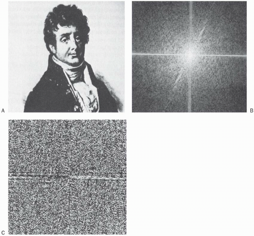 Figure 9-1. A: Picture of the French mathematician Fourier. B: The magnitude of Fourier’s two-dimensional Fourier transform. C: The phase of his Fourier transform. (Reprinted with permission from Oppenheim AV. Signals and systems. Prentice Hall; 1983.) |
 |
Example 2
The Fourier transform of this signal (Fig. 9-4) has a rectangular shape and shows that the signal
contains, not just a single frequency, but a range of frequencies from −ω0 to + ω0.
contains, not just a single frequency, but a range of frequencies from −ω0 to + ω0.
Bandwidth = ±ω0 = 2ω0 (We’ll discuss bandwidth again later.) So the Fourier transform tells us the range of frequencies that there are in a signal, as well as the amplitude of the signals at those frequencies. What’s nice about the Fourier transform is that if we have the range of frequencies and the amplitudes, we can reconstruct the original signal back.
Example 3
Let’s consider two frequencies:
cos ωt and
cos 2ωt (which is twice as fast as cos ωt)
The signal cos(2ωt) oscillates twice as fast as cos(ωt) (Fig. 9-5


Related posts:
Stay updated, free articles. Join our Telegram channel
Full access? Get Clinical Tree
