Magnetic resonance (MR) imaging of the nerves, commonly known as MR neurography is increasingly being used as noninvasive means of diagnosing peripheral nerve disease. High-resolution imaging protocols aimed at imaging the nerves of the hip, thigh, knee, leg, ankle, and foot can demonstrate traumatic or iatrogenic injury, tumorlike lesions, or entrapment of the nerves, causing a potential loss of motor and sensory function in the affected area. A thorough understanding of normal MR imaging and gross anatomy, as well as MR findings in the presence of peripheral neuropathies will aid in accurate diagnosis and ultimately help guide clinical management.
Key points
- •
Magnetic resonance (MR) imaging of the peripheral nerves is accomplished by using a combination of pulse sequences allowing detection of changes in both nerve signal and architecture.
- •
Characteristic MR imaging findings allow differentiation of neuropathic conditions related to entrapment, trauma, iatrogenic injury, extrinsic mass effect, and tumors/tumorlike lesions of the nerves.
- •
In the setting of suspected neuropathy, MR imaging findings complement clinical evaluation and electrodiagnostic testing, facilitating accurate and timely diagnosis, and promoting appropriate management.
Introduction
Magnetic resonance (MR) imaging of the nerves, also known as MR neurography (MRN), is increasingly being used as a noninvasive means of diagnosing peripheral nerve disease. Patients often present with vague symptoms, including poorly defined pain and possible functional impairment, producing a complex clinical picture. In the past, patients with perceived neurologic symptoms were referred for electromyography (EMG); however, MR imaging is increasingly being selected over other imaging modalities because of its superior soft tissue contrast, its capacity to identify and describe neural injuries, and its ability to demonstrate additional causes of nerve impairment, as well as secondary findings, such as muscle edema or denervation. MR imaging using high-resolution 2-dimensional (2D) fast spin-echo (FSE) techniques combined with fluid-sensitive sequences in the plane perpendicular to the long axis of the peripheral nerve can reveal traumatic or iatrogenic injuries, entrapment, inflammation, and tumorlike lesions affecting the nerves of the lower limb. Although the treatment for peripheral neuropathies varies based on the type of injury, region, and underlying disease, early diagnosis is essential to restore normal sensory and motor function. Studies have demonstrated that MRN findings can significantly influence the clinical management of patients with lower limb neuropathies, helping to determine which causes would benefit from surgical intervention. This article focuses on MRN of the lower limb, discussing the imaging techniques, normal anatomy, and pathologic conditions affecting the major nerves in the hip, thigh, knee, ankle, and foot.
Normal anatomy and imaging technique
General Imaging Technique
Imaging of the peripheral nerves is best performed at 1.5 or 3.0 T field strengths, with the type of coil used, the imaging planes acquired, and the scan parameters determined by the body part being imaged. Complete evaluation requires the ability to detect alterations in both nerve signal and morphology; therefore, some combination of pulse sequences providing high-resolution morphologic depiction and sensitive detection of mobile water is necessary. At the authors’ institution, general extremity imaging consists of 3-plane intermediate 2D moderate echo time FSE images plus fluid-sensitive imaging (short tau inversion recovery [STIR] or T2 with fat saturation) obtained in a single plane optimal to the structure being imaged. When specifically evaluating peripheral nerves, this general protocol is augmented by the addition of axial STIR images oriented perpendicular to the long axis of the nerve in question ( Fig. 1 ). Additional oblique coronal and sagittal images may further disclose the long axis of the nerve and the transition at points of compression. The standard matrix in the frequency direction is 512 with a phase matrix of 320 to 384. Although the field of view varies based on the body part being scanned, off-set images of the affected limb are preferred to minimize pixel size and maximize in plane resolution. Thin slices without an interslice gap further improve through plane resolution.
Other authors have described dedicated neurographic imaging protocols using sequences specifically tailored to the evaluation of peripheral nerves. Chhabra and colleagues advocate a protocol based on a combination of T2 and diffusion-weighted imaging (DWI) neurographic sequences, which includes T1 FSE, T2 adiabatic inversion recovery (IR), proton density (PD), 3-dimensional (3D) IR, and 3D diffusion-weighted reversed fast imaging with steady state precession (DW-PSIF) hybrid pulse sequences; the addition of 3D sequences with isotropic voxel sets allows multiplanar reformation, whereas the addition of hybrid DWI provides nerve-selective images with suppression of adjacent vascular structures. The administration of an intravenous gadolinium-based contrast agent is rarely warranted outside of the setting of suspected enhancing soft tissue mass lesion.
More advanced imaging techniques include diffusion tensor imaging (DTI), a technique which exploits the anisotropic properties of axonal fiber tracts and nerves, allowing the creation of fiber tract maps, as well as the calculation of quantitative parameters such as absolute diffusion coefficient (ADC). Although conventional DWI measures restriction in the Brownian motion of water by using the addition of a pair of diffusion gradient pulses before and after the 180° pulse, DTI requires the application of at least 6 diffusion gradients to detect and quantify directional diffusion along the longitudinal axes of axons. The ADC is a quantitative descriptor of diffusivity and fractional anisotropy; neuropathic conditions often result in decreased fractional anisotropy (increased ADC), whereas axons recovering from an insult often exhibit increased fractional anisotropy (decreased ADC). Although DTI provides clinically useful information, the technique is technically demanding, still somewhat experimental, and not yet adapted for routine clinical use. New gadolinium-based MR imaging contrast agents have demonstrated potential for neurographic application in animal models. For example, gadofluoride M appears to be useful in assessing demyelination and remyelination in peripheral nerves, selectively accumulating in nerves undergoing Wallerian degeneration, and dispersing when remyelination occurs.
Imaging at higher field strength is often advantageous in terms of image quality, although in certain situations, it may be detrimental. Although 3.0-T imaging results in increased signal-to-noise ratio (SNR) and superior contrast-to-noise ratio, increased field strength also results in exaggeration of certain artifacts, as well as increased energy deposition. In particular, metallic susceptibility artifact is markedly increased at 3.0 T, and patients with orthopedic implants or other hardware are universally scanned at 1.5 T at the authors’ institution. Additional considerations include alterations in tissue relaxation parameters; at higher field strengths, T1 relaxation time is prolonged, whereas T2 decay time is shortened. Imaging protocols performed at 3.0 T therefore may require longer time to repetition (TR) and shorter time to echo (TE).
Magic angle artifact affects highly ordered anisotropic structures, such as tendons and nerves, on pulse sequences with short to moderate TE when the structure in question is oriented at 55° relative to the main magnetic field (Bo). The morphology of these structures, with their highly ordered parallel fibers, augments dipole-dipole interactions involving protons within bound water, resulting in rapid dephasing, which manifests as low signal intensity on images. The strength of these dipole interactions varies with the orientation of the structure relative to Bo; at 55° to Bo, dipole interactions are minimized, resulting in relative T2 prolongation and signal hyperintensity. Although this phenomenon can be overcome by increasing the echo time (>40 ms) when imaging other morphologic structures such as tendons, the perceived high signal intensity in the nerve can persist despite slightly longer echo times and is simultaneously visualized on commonly used IR images. However, whereas magic-angle artifact may occur on neurographic imaging, Kastel and colleagues demonstrated that it rarely results in false-positive interpretation of studies, because significant magic-angle effect occurs only at angles above 30°, and that true neuropathic lesions generally result in a much greater degree of hyperintensity than can be accounted for by magic angle alone. Careful scrutiny of the nerve of interest for associated morphologic changes while remaining cognizant of the potential for magic angle phenomenon allows the interpreting radiologist to avoid false-positive interpretation in the setting of a hyperintense nerve.
MR Imaging Characteristics of Normal Nerves
In the evaluation of MR images for peripheral nerve neuropathies, it is important to have a solid understanding of the normal appearance of nerves, including their size, course, and signal intensity. On T1-weighted images, normal nerves demonstrate a fascicular appearance with intermediate signal intensity, often described as being isointense to the surrounding skeletal muscle. On STIR or fat-suppressed T2-weighted images, a normal nerve can appear slightly hyperintense as compared with the adjacent muscle tissue. Normal nerves appear to be similar in size compared with adjacent arteries (decreasing in size as one moves distally) and there is minimal to no disruption or enlargement of the fascicles. The perineural fat planes should appear preserved and the nerve should be surrounded by a hyperintense halo of perineural fat. If intravenous contrast (ie, gadolinium) is administered, normal peripheral nerves will show no enhancement. Finally, normal nerves should course smoothly and be free of sharp angulation ( Fig. 2 ).
Normal Anatomy
To properly image the nerves of the lower limb, a review of the relevant anatomy is helpful. Sensory and motor innervation of the hip, thigh, lower leg, and foot originates in the lumbosacral plexus, which is divided into 2 parts: the lumbar plexus (T12, L1–4) and the sacral plexus (L4–5, S1–4). The lumbar plexus includes the branches of the genitofemoral, obturator, lateral femoral cutaneous, and femoral nerves, with the anterior division innervating the flexors and the posterior division innervating the extensors. The sacral plexus includes the superior and inferior gluteal nerves, as well as the pudendal, sciatic, peroneal, and tibial nerves.
Obturator nerve
The obturator nerve arises from the ventral L2–L4 rami, exiting the pelvis through the obturator canal and splitting into anterior and posterior branches. The nerve innervates the anterior portion of the gracilis muscle as well as the adductor muscles of the thigh. In the pelvis, the nerve runs along the iliopectineal line and descends vertically on the obturator internus before entering the obturator canal and bifurcating. The anterior branch descends anterior to the obturator externus and adductor brevis. The posterior branch descends between the adductor magnus and adductor brevis, innervating the obturator externus and adductor magnus while providing sensation to the medial aspect of the knee joint. An accessory obturator nerve has been identified in 10% to 30% of individuals, arising from L3 or L4. When present, it innervates the hip joint and often replaces the femoral branch in the pectineus.
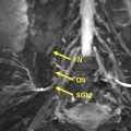
On MR imaging, the obturator nerve is well visualized in all 3 imaging planes, possibly because of the nerve’s size and abundant perineural fat. Identification of the anterior and posterior branches is easiest on axial images; the anterior branch is located in a thin area of fat, posterior to the adductor longus and anterior to the adductor brevis, whereas the posterior branch is seen within the obturator externus.
Femoral nerve
The femoral nerve is the largest branch of the lumbar plexus and provides both motor and sensory functions. The femoral nerve has extensive cutaneous distribution, starting at the anterior lateral thigh and moving distally to the medial leg and foot. Arising from the ventral L2–L4 rami, the femoral nerve lies between the psoas major and iliacus muscles. The nerve descends inferolaterally through the psoas muscle, traveling in what is commonly known as the iliacus compartment and emerging posterior to the inguinal ligament. Once in the femoral triangle, the nerve splits into multiple branches. The anterior branch has both cutaneous and muscular divisions, innervating the pectineus and sartorius muscles and controlling hip flexion and knee extension. The posterior branch of the femoral nerve is best known for its innervation of the quadriceps muscles and subsequent division to form the saphenous nerve.
On MR imaging, the femoral nerve can be visualized in all 3 imaging planes. The femoral nerve appears as a subtle projection off of the surface of the muscle on axial images and can be seen on coronal images as it courses under the inguinal ligament. The femoral nerve can also be identified by its close proximity to the femoral artery and vein throughout the hip and thigh.
Lateral femoral cutaneous nerve
The lateral femoral cutaneous nerve (LFCN) of the thigh arises from the ventral L2 and L3 rami. It is a somatosensory nerve that provides sensation to the lateral thigh and knee. Although the course of the nerve is variable, it commonly emerges anterior to the iliac crest and lateral to the psoas major, descending obliquely toward the anterior superior iliac spine. Once distal to the inguinal ligament, the LFCN divides into smaller branches that pierce the fascia lata and innervate the skin of the thigh. At the authors’ institution, the LFCN is one of the few nerves of the lower limb that requires an additional imaging sequence for proper visualization. A thin (∼1 mm) coronal package of the anterior thigh is performed to ensure adequate visualization of the LFCN, as the nerve courses horizontally in the anterior compartment. Although the nerve can be followed in the axial plane intrapelvically, it is well visualized in the coronal and sagittal planes within the thigh.
Sciatic nerve
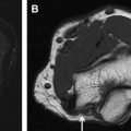
The sciatic nerve is the thickest nerve in the body, dividing into 2 distinct parts in the distal thigh: the tibial and common peroneal (fibular) nerves. Formed by the nerve fibers of the ventral L4 rami and sacral S1–S3 rami, the sciatic nerve lies anterior to the piriformis muscle. The nerve enters the thigh at the inferior border of the gluteus maximus and continues to descend posterior to the adductor magnus. Although contained by a common epineurium, the nerve splits into the tibial (anterior) and common peroneal (posterior) nerves at roughly the popliteal fossa. Similar to the obturator nerve, the sciatic nerve is easily identified on MR imaging in all 3 imaging planes because of its large size and abundant perineural fat content. High-resolution axial FSE images demonstrate 2 distinct nerve fascicles bound by a common sheath (see Fig. 2 ).
Saphenous nerve
The saphenous nerve is formed from the posterior branch of the femoral nerve and travels along the medial aspect of the distal thigh. In the leg, the saphenous nerve descends posteromedially, descending between the sartorius and gracilis muscles and supplying sensation to the infrapatellar region. The nerve continues down the medial aspect of the leg, traveling with the great saphenous vein. It descends anterior to the medial malleolus, and innervates the medial aspect of the foot. On MR imaging, the saphenous nerve is most commonly evaluated on axial PD or axial IR images through the clinically relevant area.
Tibial nerve
The tibial nerve (L4–L5, S1–S3) arises from the medial portion of the sciatic nerve. It originates at the approximate level of the popliteal fossa and travels through the posterior compartment of the leg, descending between the heads of the gastrocnemius muscle. The tibial nerve provides motor innervation to the deep and superficial posterior compartments, including muscles such as the plantaris, gastrocnemius, soleus, popliteus, posterior tibialis, flexor digitorum longus, and flexor hallucis longus. Distally, the tibial nerve becomes increasingly superficial, traveling medial to the Achilles tendon as it enters the ankle, at which point it is termed the posterior tibial nerve. The nerve descends between the flexor digitorum longus and flexor hallucis longus, before entering the foot. On the postero-inferior side of the medial malleolus, the tibial nerve gives rise to the medial calcaneal nerve(s) nerve before bifurcating to form the medial and lateral plantar nerves, the latter of which gives rise to the inferior calcaneal nerve. On MR imaging, the tibial nerve is best visualized on axial images through the leg and ankle joint. The posterior tibial nerve courses in close proximity to the tibial artery and vein, providing an easy way to trace the nerve on axial images. In the foot, the terminal branches of the tibial nerve are seen on axial images around and through the tarsal tunnel and on short-axis oblique coronal images more distally.
Common peroneal (fibular) nerve
The common peroneal nerve (CPN) arises from the lateral portion of the sciatic nerve in the distal, posterior femur. In the thigh, the CPN innervates the short head of the biceps femoris and provides sensation to the proximal lateral leg. The nerve travels inferolaterally in the popliteal fossa and descends obliquely toward the back of the head of the fibula. After winding around the lateral portion of the fibular head, the CPN trifurcates into the recurrent articular branch, superficial branch, and deep branch. The CPN can be easily visualized on MR images, because it is surrounded by a significant amount of fat. Axial images through the distal thigh and into the knee joint reveal the CPN as it moves from the short head of the biceps femoris muscle to the lateral head of the gastrocnemius. Even before physical bifurcation, the deep and superficial branches of the CPN can be visualized in the posterior distal thigh and knee joint.
Deep peroneal nerve (fibular) nerve
The deep peroneal nerve (DPN) is first identified between the fibular neck and the peroneus longus muscle. Descending in the anterior compartment of the leg, the DPN travels on the anterior surface of the interosseous membrane, lateral to the tibialis anterior. More distally, it runs between the extensor digitorum longus and the extensor hallucis longus tendons. In the leg, the DPN innervates the extensor muscles of the anterior compartment, including the tibialis anterior, extensor hallucis longus, extensor digitorum longus, and peroneus tertius muscles with little sensory innervation. At the ankle, the DPN passes under the hallucis longus tendon and the extensor retinaculum, entering the tarsal tunnel. In this region, branches of the nerve provide motor function to the extensor digitorum brevis and sensation to the first web space of the foot, ankle, and tarsal and metatarsophalangeal joints.
On MR imaging, the distal portion of the DPN is easily visualized at the knee joint using axial images. To locate the nerve more proximally, the anterior tibial artery can be used as a guide, as it is often either medial or posterior to the DPN. In the foot, short-axis images of the midfoot are often used to evaluate the medial and lateral branches; however, given the medial branch’s small size and proximity to other anatomic structures, it can be difficult to identify.
Superficial peroneal (fibular) nerve
The superficial peroneal nerve (SPN) is a branch of the CPN, coursing anterior to the fibula in the lateral compartment of the leg and providing motor function to the peroneus longus and brevis as well as sensation to the anterolateral leg. More distally, the nerve becomes subcutaneous and pierces the deep fascia on the anterior surface of the lateral compartment. The SPN then divides above the lateral malleolus into 2 distinct branches: the intermediate and medial dorsal cutaneous nerves. On MR imaging, axial images are often best for tracing the course of the SPN. At the level of the knee, the SPN can be identified as the more posterior portion of the CPN. More distally, the nerve can be identified in a thin area of fat between the muscles of the anterior and lateral compartments of the leg. The SPN is also well visualized through the ankle and foot as long as images are acquired perpendicular to the long axis of the nerve.
Sural nerve
The sural nerve is a sensory nerve formed from the medial sural cutaneous nerve (branch of the tibial nerve) and lateral sural cutaneous nerve (branch of the CPN). The sural nerve courses in the posterolateral leg, lateral to the Achilles tendon. More distally, the nerve travels superficial and posterior to the peroneal tendons, producing a branch to the heel and then terminating in the lateral foot. The sural nerve provides sensation to the lateral foot and heel via the lateral calcaneal nerve and lateral dorsal cutaneous nerve branches. On MR imaging, the sural nerve is best located at the lateral margin of the Achilles tendon and calcaneus, and courses adjacent to the often prominent lesser saphenous vein.
Medial plantar nerve
The medial plantar nerve is a terminal branch of the tibial nerve. Homologous to the median nerve in the hand, the medial plantar nerve courses medially in the foot with the medial plantar artery. In the sole of the foot, the nerve can be found between the muscle of the abductor hallucis and the flexor digitorum brevis, traveling between the first and second layers of the plantar muscles. The medial plantar nerve provides motor innervation to the abductor hallucis, flexor digitorum brevis, flexor hallucis brevis, and lumbricals. On MR imaging, the medial plantar nerve is best visualized on thin axial images through the ankle and foot as well as far medial sagittal images through the foot.
Lateral plantar nerve
The lateral plantar nerve is the smaller of the 2 terminal branches of the tibial nerve. Homologous with the ulnar nerve in the hand and wrist, the lateral plantar nerve travels anterolaterally within the second plantar layer. Branches of the lateral plantar nerve innervate the abductor digiti minimi and flexor accessorius (quadratus plantae). The nerve also provides motor function to the 3 lateral-most lumbricals, as well as the dorsal and plantar interosseous muscles. It provides sensory innervation to the lateral aspect of the foot and toes. At the medial portion of the base of the fifth metatarsal, the lateral plantar nerve divides into superficial and deep branches. Similar to the medial plantar nerve, the lateral plantar nerve is best visualized on MR imaging using thin axial images through the area of clinical interest.
Medial and inferior calcaneal nerves
The medial calcaneal nerve arises from the posterior portion of the tibial nerve. The nerve pierces the flexor retinaculum and subsequent branches provide sensory innervation to the posteromedial heel as well as the medial side of the sole of the foot and the plantar fat pad. The inferior calcaneal nerve, also known as the Baxter nerve, has been shown in cadaveric studies to originate from the lateral plantar nerve at the level of the medial malleolus. The nerve travels between the abductor hallucis and the quadratus plantae along the medial aspect of the long plantar ligament. In the hindfoot, the inferior calcaneal nerve makes a sharp 90° turn from vertical to horizontal as it travels laterally to supply the abductor digiti minimi. The inferior calcaneal nerve provides motor function to the abductor digiti quinti muscle and the flexor digitorum brevis and provides sensation to the long plantar ligament and the heel of the foot. On MR imaging, the inferior calcaneal nerve is most easily identified on coronal intermediate weighted or axial IR images through the area of clinical interest. This nerve can be traced as it branches off of the lateral plantar nerve and descends toward the abductor digiti minimi.
Related posts:
 MR Neurography
 High-Resolution Magnetic Resonance Neurography in Upper Extremity Neuropathy
Magnetic Resonance Neurography Research
High-Resolution Magnetic Resonance Neurography in Upper Extremity Neuropathy
Magnetic Resonance Neurography Research
 Magnetic Resonance Neurography of the Pelvis a nd Lumbosacral Plexus
 High-Resolution Magnetic Resonance Neurography in Upper Extremity Neuropathy
 Peripheral Nerve Surgery
Stay updated, free articles. Join our Telegram channel

Full access? Get Clinical Tree


