(1)
MGH Department of Radiology, Harvard Medical School, Newton, MA, USA
Abstract
Some 20 years ago, when I was starting my student research in image compression, my more advanced friends kept asking me, why on earth I chose to burden myself with such an antiquated and useless subject. Disk storage was growing rapidly, network bandwidth was rising, and dialup modems were firing data with “lightning-fast” 14 kb/s. Why compress, when we’ll be able to handle everything uncompressed in a year?
Key Points
Image compression is in constant demand as the only practical way to deal with ever-growing imaging data volume. Lossless compression does not change the original image, but achieves rather modest 2–4 compression factors. Lossy compression can typically reduce data volume by 10–20 times, but you need to be aware of the irreversible artifacts that it introduces into the images. This chapter explains the mechanics of compression and their impact on diagnostic imaging.
4.1 Why Even Bother?
Some 20 years ago, when I was starting my student research in image compression, my more advanced friends kept asking me, why on earth I chose to burden myself with such an antiquated and useless subject. Disk storage was growing rapidly, network bandwidth was rising, and dialup modems were firing data with “lightning-fast” 14 kb/s. Why compress, when we’ll be able to handle everything uncompressed in a year?
But that year passed by, and then another, and by the time I joined my first Radiology department the folks around me were screaming from the data volume overdose. It turned out that the wonderful “larger storage, faster network” argument somehow missed its most essential counterpart: exploding data sizes. Clinical data volumes – medical imaging in particular, as the most megabyte-hungry – went through the hospital roofs, turning data storage and transmission into the most expensive enterprise of the digital age. Consequently, data compression has become an integral part of modern medical workflow, even if you never thought about it before. In fact, you can get yourself into serious trouble if you keep ignoring compression, as most of us did and still prefer to do. So let’s spend some time studying how it works, and how it changes your diagnostic images.
4.2 Lossless Compression
“Sure, I know how image compression works,” you say. “It removes image pixels to make the image smaller!”
My dear interlocutor, you cannot even imagine how many times have I heard this brave answer. It’s kind of natural to assume that to make something smaller you have to trim it down, but nothing could be further from reality in the case of image compression.
Contrary to popular belief, compression is the art of rewriting the original information in the most condensed form. Think about a hypothetical “Compressian” language, so laconic that translation into it always results in much shorter sentences and fewer letters. For example, imagine that you have a sequence S1:
a a a a a b b b b b b b
which you “translate” into sequence S2:
5a 7b
meaning that ‘a’ needs to be repeated five times, and ‘b’ – seven. Both sequences S1 and S2 are identical – they say exactly the same thing – but the second one is much shorter: you have 4 characters instead of the original 12, thus compressing the S1 data with a 3:1 compression ratio.1 This simple compression algorithm is known as run-length encoding (RLE) – we replace repetitive symbols (or numbers, or even entire words) by their counts. You may think that the example is a bit far-fetched; after all, who uses repetitive letters in a textual sentence? True enough, but who said that we have to compress text only? Think about images, where entire pixel lines may be equal to the same background color. Then instead of storing long sequences of identical pixels, we can apply RLE, instantly reducing the original data size.
As a result, RLE works great if the repetitive patterns are sequential. But one can do even better, exploring non-sequential redundancies. Moreover, you might be doing this daily without paying any attention to it. For instance, if you need to text sentence S3:
You know that you are what you eat
and you don’t have much time, you could type it as S4:
u know that u r what u eat
which is definitely shorter than S3. You simply picked the most frequently-used words – such as “you” and “are” – and replaced them with the shortest possible codewords, “u” and “r”. Presto! You’ve built a simple compression dictionary (Table 4.1).
Table 4.1
Simple compression dictionary
Original pattern | Codeword |
|---|---|
you | u |
are | r |
It’s obvious that if you keep replacing the most frequent patterns with shortest possible codewords, you will shorten the data in the most efficient way; just make sure that your codewords are unique and cannot be parts of each other (a concept known as prefix coding,2 just as you see it in country calling codes). This is precisely what most frequency-based compression techniques do, whether it is LZW compression3 used to make ZIP files, or Huffman compression4 employed to compress images. These algorithms may rely on more advanced approaches to achieve the optimal encoding, but the essence of compression is the same: replacing the most redundant patterns with the shortest codewords does the job.
These trivial examples teach us a few valuable lessons:
Compression attempts to encode the original data in the most compact form. This encoding is reversible: the original data can be fully recovered from its compressed representation (you can recover S1 from S2, or S3 from S4, without losing anything “in translation”). Therefore reversible compression is also known as lossless.
Any compression is about exploring the original data redundancy. High redundancy (substantial presence of repetitive patterns) helps you achieve higher compression rates. Low redundancy (unpredictable patterns), on the contrary, makes data harder, if not impossible, to compress.
Compression is quantified by compression ratio . Thus, for our RLE example with S1 and S2, R c = 3.
To translate the original into “Compressian”, compression builds encoding dictionaries, replacing long repetitive patterns by short dictionary codewords. For instance, our dictionary in {S3, S4} is shown in Table 4.1. Applying the dictionary in the reverse direction uncompresses S4 back into S3.
Compression requires data processing: the computer has to find the most repetitive strings and replace them with the codewords; in some instances, it may have to compute the optimal codewords.5 Processing takes time, and spending this time on compressing/uncompressing is the flip side of any compression implementation.
With these lessons learned, there is really nothing mind-blowing about the basic compression principles. Rest assured that none of them removes pixels from the original image data. Moreover, lossless compression can do a great job in many cases, with typical R c ranging from 2 to 4. But this lossless idyll quickly fades when one runs into mega- and gigabytes of data (image databases, device raw data, high-resolution scans, large-scale projects). In this case we need at least an order of magnitude R c before our workflow becomes remotely practical. We need to go lossy.
4.3 Lossy Compression
One image pixel takes roughly the same memory as one letter. Now imagine that you have to store a CT image exam (500 images, for instance) along with some textual data of, say, 10,000 letters (patient demographics, history, report). Ten thousand letters may seem like a lot, but a standard 512 × 512 CT image has 512 × 512 = 262,144 pixels, which is already 26 times the size of the accompanying text. Now, if you multiply 26 by 500 images, you should get the full picture: medical images take a lot more space than medical text does.
So we need to target the images, and we need to compress them very efficiently. Just as we discussed earlier, images are sequences of pixels. One can read them line by line, starting from the top left pixel. Therefore lossy compression applies as usual: if we have a sequence S5 of pixel values with something like:
1000 1000 1000 1003 1002 1005 1576 1623 1627 1620…
we can definitely apply RLE or LZW to compress it – for instance, replacing the values of 1000 with a shorter codeword “x” to build a compressed S6:
3x 1003 1002 1005 1576 1623 1627 1620…
This looks good, but for most images this would yield R c around 2: good enough to save on disk storage, but hardly enough to send that CT case to a smartphone in real-time, over a jammed network. Can we compress any stronger?
Yes, if we adopt the idea of irreversible lossy compression, achieving higher R c through slight alterations in the original pixel values. Indeed, the difference between pixel values of 1000 and 1003 in S5 may not have any diagnostic meaning. You may not even be able to perceive this difference at all. If this is the case, we can define a pixel error threshold ε – “perceptual error” – and consider all pixels within this threshold equal. For instance, if we choose ε = 5, then the original S5 can be replaced by S7 such that:
1000 1000 1000 1000 1000 1000 1576 1623 1623 1623…
This definitely increases the degree of redundancy, so that we can compress S7 as S8:
6x 1576 3y…
– a much better result compared to S6.
Nota bene:
Note that in some cases, lossy compression is not an option. Consider text: we cannot pretend that the letters ‘a’ and ‘b’ are “close enough” to be interchangeable. We can afford to replace something only when the replacement doesn’t matter to us.
Thus, lossy compression typically includes two distinct steps: approximating the original data samples with some admissible error ε to increase data redundancy, and compressing the approximate values with conventional lossless compression. When the approximation is exact (ε = 0) we get our standard lossless case of nothing being lost or altered. It is when ε > 0 that we lose the reversibility: one cannot recover S5 from S7.
Thus begins the whole “lossy vs. diagnostic” argument: how much ε roundoff can we tolerate without losing diagnostic image quality? Think about setting ε = 700 – then all ten pixel values in S5 can be rounded to 1000, and the sequence will be compressed as 10x. This is a remarkably high compression ratio, but with all image detail totally lost! So we really want to stop somewhere in the middle between ε = 0 and ε = “Gee, the image is gone!” – to preserve original diagnostic image quality while keeping the data size as small as possible.
This is exactly where lossy compression becomes more of an art. Suffice it to say that the differences between image pixel values can be diagnostic in some cases (such as tiny micro-calcifications in mammograms), and purely meaningless in others (such as noise in low-dose X-ray or CT images). Consequently, the same values of ε can be too high for one image (or image area, or specific malignancy) and way too low for another. Moreover, pixel value fluctuations can depend on different tissue types, image acquisition protocols, imaging artifacts, and so forth. As a result, there is no universally-perfect ε for diagnostically-safe lossy compression, and there is no universally-perfect R c to ensure that your lossy image will stay flawless. Most literature on this matter seems to be strangely attracted to R c = 10, but some suggest 15–20 (Kim et al. 2012), 70 (Peterson and Wolffsohn 2005), or even R c = 171 (Peterson et al. 2012),6 while the others advise caution even at R c = 8 (Erickson et al. 2010) – always specific to the images, circumstances, experiences7 or even countries (Table 4.2) (Loose et al. 2009), without any guarantee that the same R c will work for you. This leaves you with only one real option: trying it yourself. If you are using lossy compression – inevitable in projects like teleradiology – you will need to experiment with different compression settings provided in your software to see that the diagnostic integrity of your images remains intact.8
Table 4.2
Summary of recommended compression rates in Canada, England, and Germany
Canada | England | Germany | |
|---|---|---|---|
Radiography | 20–30 | 10 | 10 |
Mammography | 15–25 | 20 | 15 |
CT | 8–15 | 5 | 5–8 |
MR | 16–24 | 5 | 7 |
RF/XA | n/a | 10 | 6 |
Nota bene:
Keep in mind that there is absolutely no straightforward way to associate compression ratio R c with compressed image quality; the latter depends on many objective and subjective factors such as image texturing or human vision phenomena, generally ignored by the compression algorithms. But compression ratio works perfectly well when we talk about data size reduction – this is precisely what R c means, and this is why it is so much appreciated.
To carry out this task of identifying compression artifacts, we need to look at them more closely.
4.4 JPEG Artifacts
JPEG compression and image format have been around since the 1990s, and have gained enormous popularity with many applications, including early adoption by the DICOM standard (Pianykh 2005). Instead of ε-thresholding that we discussed earlier, JPEG takes a different route. First, it breaks an image into 8 × 8 blocks to localize image features, and approximates each block in 2D by representing it as a weighted sum of predefined 8 × 8 intensity patterns (“codewords”, based on Discrete Cosine Transform functions, or DCT,9 Fig. 4.1). Then, instead of storing the original 8 × 8 = 64 pixel values in each block, JPEG needs to store only a few weighting coefficients, required for the block’s DCT decomposition – and that’s how the compression magic is done. This is a good way to explore image redundancies: first of all, we take full advantage of the 2D image format; second, naturally-smooth images will require only a few top DCT coefficients per block, leading to high compression ratios.
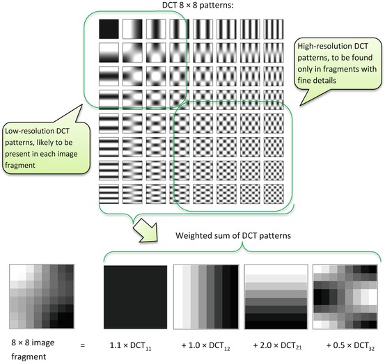

Fig. 4.1
JPEG uses predefined DCT image patterns to represent each 8 × 8 fragment of the original image. If we can approximate the fragment with only a few DCT patterns, then all we need to store is the pattern coefficients, such as {1.1, 1.0, 2.0, 0.5} in our example. Storing those few coefficients instead of the original 64 pixels is the key idea behind JPEG compression
Inversely, when the images get noisy, or block boundaries run across some image edges (such as sharp intensity changes between different organs), JPEG magic starts falling apart. And when this happens, JPEG’s 8 × 8 blocks will be right in your face – then you’ll know the tiger by its tail. Why does JPEG have this artifact? To achieve high R c , JPEG has to sacrifice the heaviest ballast of its higher-order DCT coefficients, the ones responsible for the fine image details. Thus, only the less numerous, least-detailed patterns survive, resulting in dull and disconnected checkerboards (Fig. 4.2, right).
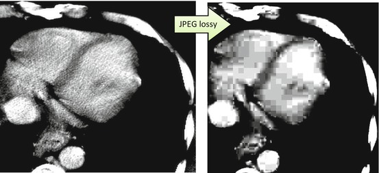

Fig. 4.2
Too much of JPEG’s lossy compression will leave you with severe blocking artifacts. Note that all fine texture details, present in the original image (left), are gone in the compressed image (right). R c = 20
It’s important to know that the JPEG compression standard has several advanced flavors, lossless included. You can find them in DICOM software (often used on CT and MR scanners), but they won’t be supported in popular imaging applications such as web browsers or image editors. So bear in mind that using JPEG in your online photo album will always imply baseline lossy compression – even if you set JPEG image quality to the highest possible.
In addition to that and probably due to its venerable age, JPEG supports only 8-bit and 12-bit pixel grayscales. This means that you can have only up to 28 = 256 or 212 = 4,096 shades of gray in your medical image, depending on the flavor of JPEG you are using. DICOM, on the contrary, supports deeper 16-bit grayscale. This matters because putting a DICOM image into JPEG may bring to mind that old joke Procrustes played on his unfortunate guests. If you want to store a 16-bit-deep X-ray in a standard browser-compatible 8-bit JPEG, you will have chop off half of the original image grayscale depth, 8 = 16 − 8 bits. In plain terms it means that each 256 shades of the original image will be collapsed into a single procrustean shade of your JPEG. This will certainly wipe out many diagnostic features; don’t be surprised if you get a single color per body part.
Nota bene:
Keep in mind that compression is yet another application layer added to your imaging workflow. As such, it may have problems of its own – and oh, yes! – its own bugs. I have seen hospitals where poor JPEG implementations were simply corrupting the images.
Why this is possible, you may ask? Writing compression code is not easy, and requires substantial subject expertise. Therefore most vendors prefer to get prêt-à-porter compression libraries. You can either buy them from professional companies (which implies costs and royalties), or adopt some (nearly-) free public solutions. The latter are typically found online, or borrowed from research projects that were never meant to work on a commercial-grade scale. So after processing 1000 images successfully, they inevitably fail on image 1001, simply because their original developers (long gone) never thought of testing this many.
4.5 JPEG2000 Artifacts
JPEG2000 compression, just as its name suggests, appeared on the wake of the new millennium, as a “new generation” JPEG. Just like JPEG, JPEG2000 takes the same image-decomposition approach, shown in Fig. 4.1, so that it can store a few coefficients instead of many pixels. But unlike its DCT-driven predecessor, JPEG2000 decomposes images with wavelets – another set of cleverly designed functions – invented to represent feature-rich data. The key point about wavelets is their ability to capture local image details (such as edges and little structures) without artificially breaking the images into the 8 × 8 blocks.
This property, along with many other mathematically-optimal properties of the wavelet transform, made JPEG2000 a long-awaited compression favorite; and it does do very well in many medical apps. Moreover, JPEG2000 has no problem accommodating 16-bit pixels of your medical DICOM images, with lossy image quality usually superior to that of JPEG (Shiao et al. 2007; Gulkesen et al. 2010). But as always, overdoing its lossy compression leads to diagnostically-unacceptable artifacts, shown in Fig. 4.3; instead of JPEG’s blocking, JPEG2000 can result in substantial image blur. It happens for the same reasons: when JPEG2000 has to achieve high R c , it starts sacrificing the fine local details, as taking the most memory to store. The strategy inevitably results in blurred, detail-less areas, very much like we saw with our good old friend, JPEG.
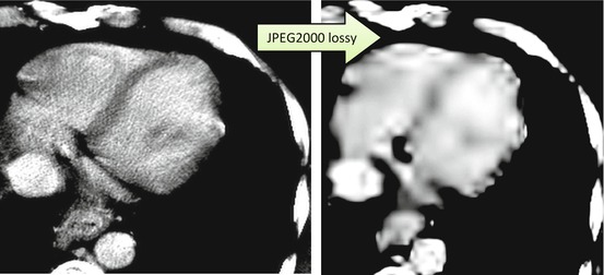

Fig. 4.3
Overdoing lossy JPEG2000 results in blur with blobbing around the edges. R c = 20
Another theoretically useful functionality explored by JPEG2000 authors was the ability to encode and stream different image regions using different strengths of compression (R c ). It was expected that this would significantly reduce the volume of data being downloaded: if the user is only going to look at a specific area, only this area needs to be transmitted with the highest quality. Unfortunately, this approach proved to be somewhat controversial: as more and more regions and details were streamed to the user, the image on the user side would keep updating itself, changing in quality and resolution. Virtually any radiologist would prefer to have the final image first, before even glancing at it.
4.6 JPEG-LS and Diagnostic Compression
Stay updated, free articles. Join our Telegram channel

Full access? Get Clinical Tree


