Image Construction: Part I (Slice Selection)
Introduction
The signals received from a patient contain information about the entire part of the patient being imaged. They do not have any particular spatial information. That is, we cannot determine the specific origin point of each component of the signal. This is the function of the gradients. One gradient is required in each of the x, y, and z directions to obtain spatial information in that direction. Depending on their function, these gradients are called
The slice-select gradient
The readout or frequency-encoding gradient
The phase-encoding gradient
Depending on their orientation axis they are called Gx, Gy, and Gz. Depending on the slice orientation (axial, sagittal, or coronal), Gx, Gy, and Gz can be used for slice select, readout, or phase encode.
A gradient is simply a magnetic field that changes from point to point—usually in a linear fashion. We temporarily create magnetic field nonuniformity in a linear manner along all three axes to obtain information about position.
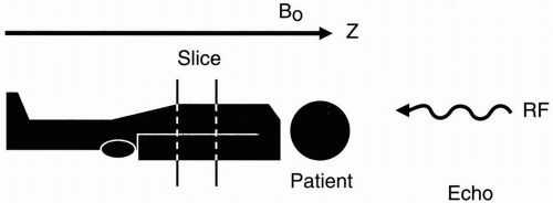 Figure 10-1. Selecting a slice of a certain thickness. |
First, we’ll consider the slice-select gradient, which is the easiest of all to understand. Once a slice has been selected, we worry about the problem of in-plane spatial encoding, that is, discriminating position within the slice. As we’ll see shortly, the principles behind slice selection and spatial encoding in MRI are different from the principles used in computerized tomography (CT).
How to Select a Slice
Suppose that we have a patient on the table and we want to select a slice at a certain level and of a certain thickness (Fig. 10-1). Remember that the patient is lying in the external magnetic field B0, which is oriented along the z-axis. If we transmit a radio frequency (RF) pulse and get a free induction decay (FID) or an echo back, the received signal would be from the entire patient. There is no spatial discrimination. All we get is a
signal, and we have no idea yet from where exactly in the body the signal is coming.
signal, and we have no idea yet from where exactly in the body the signal is coming.
The frequency of the RF pulse is given by the Larmor frequency:
ω0 = γB0
If we transmit an RF pulse that does not match the Larmor frequency (the frequency of oscillation at magnetic field B0), we won’t excite any of the protons in the patient.
However, if we make the magnetic field vary from point to point, then each position will have its own resonant frequency. We can make the magnetic field slightly weaker in strength at the feet and gradually increase in strength to a maximum at the head (Fig. 10-2). This effect is achieved by using a gradient coil.
Let’s say the magnetic field strength is 1.5 T at the center, 1.4 T at the feet, and 1.6 T at the head. Then, the foot of the patient will experience a weaker magnetic field than the head. Therefore, a gradient in any direction (x, y, or z) is a variation in the field along that axis in some fashion (the most common form of which is linearly increasing or decreasing). If we now transmit an RF pulse of a single frequency into the patient, we will receive signals corresponding to a line in the patient at the level of the magnetic field corresponding to that frequency (according to the Larmor frequency), but it will be an infinitely thin line. What we need to do is transmit an RF pulse with a range of frequencies—a bandwidth of frequencies.
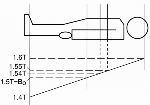 Figure 10-2. Slice thickness is determined by the slope of the gradient. |
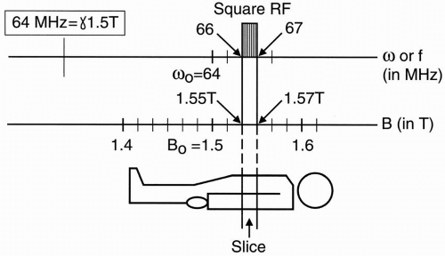 Figure 10-3. The relationship between field strength and Larmor frequency in determining slice thickness and position. |
What will the RF pulse look like in the frequency domain? First, note that for a 1.5-T magnet, the Larmor frequency is 64 MHz for hydrogen protons:
64 MHz corresponds to B0 of a 1.5-T magnet.
To see how this is derived, recall that
ω0 = γB0
where γ ≅ 42.6 MHz/T and B0 = 1.5 T This results in ω0 = 42.6 × 1.5 = 64 MHz The graph in Figure 10-3 shows the magnetic field strength and the corresponding Larmor
frequency range. We are concerned here about a magnetic field strength ranging from 1.4 to 1.6 T because, in our example, that is the magnetic field strength range to which we have exposed the patient. Let’s excite one slice with an RF pulse. For example, let’s excite a slice extending from 1.55 to 1.57 T. This corresponds to a frequency range from 66 to 67 MHz.
frequency range. We are concerned here about a magnetic field strength ranging from 1.4 to 1.6 T because, in our example, that is the magnetic field strength range to which we have exposed the patient. Let’s excite one slice with an RF pulse. For example, let’s excite a slice extending from 1.55 to 1.57 T. This corresponds to a frequency range from 66 to 67 MHz.
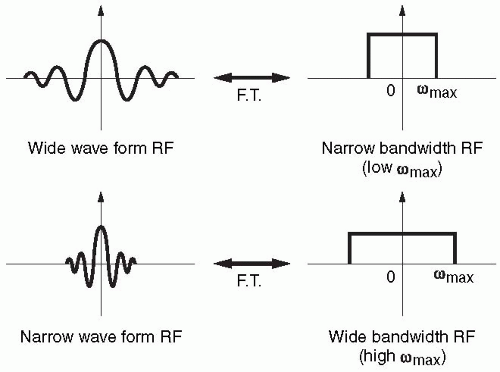 Figure 10-4. Comparison of wide and narrow waveforms and their FTs. The narrower the waveform in time domain, the wider its FT will be. |
If the RF has a square shape in the frequency domain with a range of frequencies that correspond to a range of magnetic field strengths, then we will excite only the protons that are in the slice containing that range of magnetic field strengths. The other protons in the rest of the body are not going to get excited because the range of frequencies from which we are transmitting the RF pulse does not match the Larmor frequencies of the other protons. The range of frequencies in the RF pulse will only match the Larmor frequency of a single slice.
So, we transmit an RF pulse with a range of frequencies that we know will correspond to a range of magnetic field strengths in a particular slice. This range of frequencies determines the slice thickness and is referred to as the bandwidth.
Bandwidth = range of frequencies (determines the slice thickness)
We can measure the bandwidth (range of frequencies) by looking at the Fourier transform of the RF pulse. Let’s now compare the RF signal with its Fourier transform. The RF pulse is generally a sinc wave and looks like Figure 10-4a with the Fourier transform that has a square shape.
If we have a narrower signal, we get a wider frequency bandwidth (Fig. 10-4b). The narrower signal reflects the fact that there are more oscillations in a given period of time so that the maximum frequency of the signal is greater. Because the Fourier transform depicts an infinite number of frequencies from zero to maximum, the bandwidth gets wider to depict a greater maximum frequency.
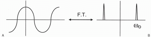
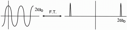
Let’s apply this example to a cosine wave (Fig. 10-5a). The Fourier transform for this cosine wave contains two spikes, one on each side of zero (Fig. 10-5b). If we then take a cosine wave with twice the oscillation frequency and look at its Fourier transform, we see that the spikes are farther apart (Fig. 10-6). Thus, as the cosine wave goes two times faster, the Fourier transform shows that the maximum frequency (in this case, the only frequency) is two times farther away from the zero point. Furthermore, if we look at the diagram of the cosine waves, the faster cosine wave has a narrower oscillating waveform—the narrower the waveform, the faster the oscillation frequency. Again, the narrower the waveform of the RF signal, the wider its bandwidth (the greater the maximum frequency; Fig. 10-6).
Slice Thickness
Let’s now talk about how we establish slice thickness (Fig. 10-7). The same principle would apply if we were to image from the base of the skull to the vertex rather than from the patient’s head to toe. We establish a magnetic field strength gradient so that at the midpoint of the field of study (in this instance, the entire body), the field strength is 1.5 T; at the low end of the gradient (the foot), the field strength will be 1.4 T; and at the high end of the gradient, the field strength will be maximum at 1.6 T. These magnetic field strengths also correspond to different frequencies. Using the Larmor equation, we can calculate that approximately:
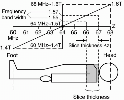 Figure 10-7. An example of the relationship between slice thickness and position, frequency, and field strength. |
 Figure 10-8.
Get Clinical Tree app for offline access
Related posts:Stay updated, free articles. Join our Telegram channel
Full access? Get Clinical Tree


|