Image Quality

4.0 INTRODUCTION

At a fundamental level, image quality is about diagnostic accuracy, which is a difficult quantity to measure. Because of this, most image quality measures are based on surrogate measures that are linked, by assumption, to task performance. Optimal image quality typically requires balancing image resolution, contrast, and noise along with other considerations such as dose or cost. The results of image quality assessments are typically a ratio measure (CNR or SNR) or a performance curve (contrast-detail or ROC).

4.1 SPATIAL RESOLUTION

Spatial resolution describes the level of detail that can be seen on an image with low-resolution images appearing “blurry” and high-resolution images appearing “sharp.”

1. Physical mechanisms of blurring
- a. X-ray focal spot blur
- b. Positron diffusion
- c. Optical diffusion in a phosphor-based detector
- d. Image processing for noise control—smoothing operations that employ averaging

2. Convolution—a mathematical way to describe blurring

a. Involves a blurring kernel that integrates over position (Fig. 4-1)
b. Assumes that the blurring operation is shift-invariant
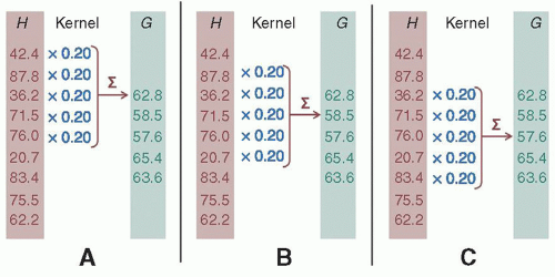
c. Can be used to smooth noisy data (Fig. 4-2)
d. Smoothing can reduce the effects of noise but can also blur fine structure in images

e. Convolution formula (see Fig. 4-1 caption for description of equation variables):

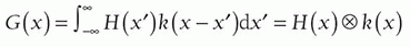
▪ FIGURE 4-1 The basic operation of discrete convolution is illustrated. In the three panes (A-C), the input array H is convolved with a five-element boxcar kernel, k, resulting in the output array, G. The different panes show the convolution kernel, and the output value, advancing by one index element at a time. The entire convolution is performed over the complete length of H.

▪ FIGURE 4-2 A plot of the noisy input data in H(x), and of the smoothed function G(x), where x is the pixel number (x = 1, 2, 3, …). The first few elements in the data shown on this plot correspond to the data illustrated in Figure 4-1. The input function H(x) is random noise distributed around a mean value of 50. The convolution process with the boxcar average results in substantial smoothing, and this is evident by the much smoother G(x) function that is closer to this mean value.

3. The spatial domain: spread functions

a. Blurring can be characterized by a point-spread function (PSF) (Fig. 4-3), a line-spread function (LSF) (Fig. 4-4), or an edge-spread function (ESF), as compared in Figure 4-5.

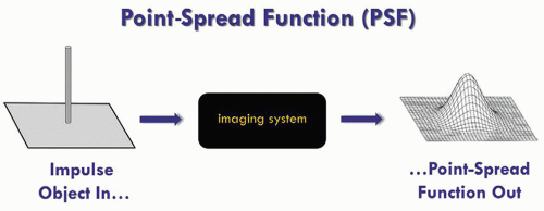
▪ FIGURE 4-3 A point impulse stimulus (left) to an imaging system (middle) and the response, the PSF (right), are shown. F. 4-4

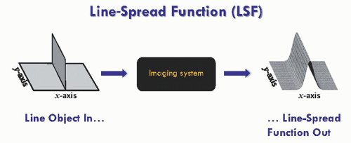
▪ FIGURE 4-4 A line impulse stimulus (left) to an imaging system (middle) and the response, the LSF (right), are shown. F. 4-7
b. These are generated by imaging a point, a slit (line), or an edge (Fig. 4-5).

c. Integral relationships exist between each of these spread functions.

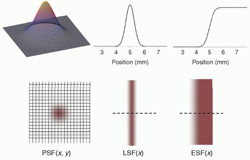
▪ FIGURE 4-5 The three basic spread functions in the spatial domain are shown—the PSF (x,y) is a 2D spread function. The LSF(x) and ESF(x) are both 1D spread functions and are related to the PSF by the convolution equation (this assumes circular symmetry):

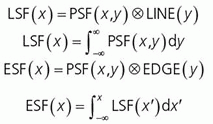
See text (Pg. 80) for details of these relationships.

F. 4-9

4. The frequency domain: modulation transfer function

a. Fourier analysis describes how a signal variation in the spatial domain can be approximated by sine waves assembled with a spatial frequency, phase, and amplitude as shown in Figure 4-6.

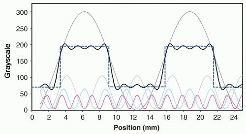
▪ FIGURE 4-6 The basic concept of Fourier analysis demonstrates how a spatial domain object (the dashed line rectangle [RECT] functions) can be estimated by the summation of sine waves. The solid black lines are the sum of the four sets of sine waves (shown toward the bottom of the plot) and approximate the two RECT functions (dashed lines). With higher frequency waves, the RECT functions could be better matched. The Fourier transform breaks any arbitrary signal down into the sum of a set of sine waves of different phase, frequency, and amplitude.

F. 4-10

b. The Fourier transform converts an image from the spatial domain to the frequency domain.
c. The Fourier transform of a sinusoidal wave function is an impulse at the wave frequency.
d. The period of a wave is the distance of one cycle; for example, period (mm)= 1/ frequency (cycles/mm).
e. Fine-scale image structure is typically reflected by high frequency content in the Fourier transform.

f. The modulation transfer function (MTF) describes how sine-wave components are modulated by an imaging system (Fig. 4-7).

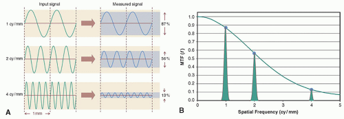
▪ FIGURE 4-7 A. Sinusoidal input signals incident on a detector at three frequencies are shown as input functions, and the measured output signals after passing through the imaging device. Input and output frequencies are the same but the amplitude of the measured signals are reduced (modulated) by resolution losses in the imaging system. B. The amplitude reduction as a function of spatial frequency is the modulation transfer function (MTF(f)). System resolution is often characterized by an MTF threshold (e.g., MTF = 10%) called the limiting spatial resolution. In this MTF, the limiting resolution would be 4.3 cycles (or line pairs/mm).

F. 4-11

g. Sampling describes the mathematical process of going from a continuous function to finite set of measured values; sampling aperture, a, and sampling pitch, Δ, are described (Fig. 4-8).

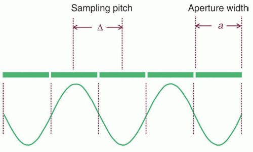
▪ FIGURE 4-8 Side view of flat-panel detector elements shows a side view of the detector elements of width, a, and the distance between the center-to-center spacing, Δ. The sampling pitch affects aliasing in the image, while the aperture width affects the spatial resolution (LSF and MTF).

F. 4-13

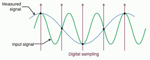
▪ FIGURE 4-9 Aliasing of the input signal as the measured signal is illustrated when the required sampling rate falls below 2 samples per cycle. The input sine wave frequency (green) is greater than the Nyquist frequency, and the sampled data will be aliased as a measured signal of lower frequency.

F. 4-14

h. Sampling at a fixed pixel pitch leads to fundamental limits on the resolution of the sampled signal.
i. Nyquist frequency = 1/2Δ (at least two samples per cycle of the input signal) is the maximum frequency that can accurately rendered in the image; when violated, aliasing occurs (Fig. 4-9).

j. Frequencies larger than the Nyquist frequency are reflected as lower frequencies (Fig. 4-10).

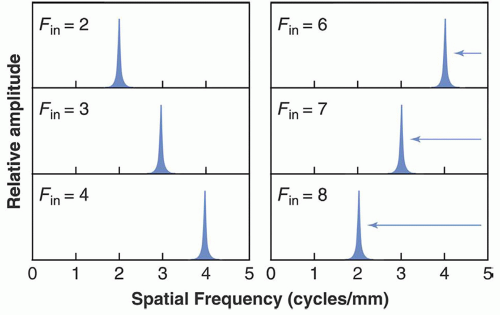
▪ FIGURE 4-10 For a single-frequency sinusoidal input function to an imaging system (sinusoidally varying intensity versus position), the Fourier transform of the image results in an impulse at the measured frequency. The Nyquist frequency in this example is 5 cycles/mm. For the three input frequencies in the left panel, all are below the Nyquist frequency and obey the Nyquist criterion, and the measured (recorded) frequencies are exactly what was input into the imaging system. On the right panel, the input frequencies were higher than the Nyquist frequency, and the recorded frequencies in all cases were aliased—they wrapped around the Nyquist frequency—that is, the measured frequencies were lower than the Nyquist frequency by the same amount by which the input frequencies exceeded the Nyquist frequency.

F. 4-15

4.2 CONTRAST RESOLUTION

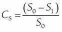
Contrast resolution refers to the ability to render subtle differences in displayed image grayscale. Contrast, C_S, is defined in terms of a background intensity, S₀, and a target intensity, S₁:

Contrast is evaluated at multiple stages during imaging (subject contrast, detector contrast and image contrast)

1. Subject contrast is the contrast in the signal after interacting with the patient (Fig. 4-11).

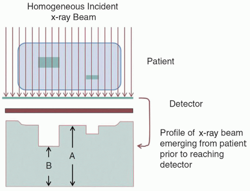
▪ FIGURE 4-11 Projection radiography example illustrates the uniform incident beam upon the patient. X-rays interact with the tissues through various mechanisms (Chapter 3) resulting in a greater differential attenuation caused by a structure (B) compared to the attenuation of the surrounding tissue (A). In this case, B (e.g., bone) is more attenuating than A (e.g., soft tissue), and S₀>S₁, thus contrast ranges from 0% to 100%. For less attenuating structures (e.g., air pockets), negative contrast is also possible. Subject contrast also has intrinsic and extrinsic factors that relate to anatomical or functional changes—intrinsic from physical or physiological properties such as a pulmonary nodule in a lung—extrinsic from acquisition protocols (e.g., changing to lower kV to emphasize ribs for a rib radiograph, or to higher kV to de-emphasize the ribs for a chest x-ray), or introducing iodinated contrast agent to identify the location of the vasculature or perfusion uptake in an organ.

F. 4-17

2. Detector contrast transduces the incident signal through many possible processes that impact the contrast of structures of interest (Fig. 4-12).

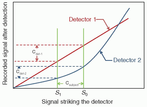
▪ FIGURE 4-12 Characteristic curve response of two detector systems maps the signal striking the detector (x-axis) into a recorded signal (y-axis). A linear response for detector 1 and a nonlinear response for detector 2 shows the subject contrast signals (S₁ and S₀) are a consequence of the characteristic curve of the detector. In this case, the detector contrast for detector 1 at the level of the input signals is larger than for detector 2.

F. 4-18

3. Image contrast
- a. Capture of digital image data allows for interactive adjustment of image contrast through window/level manipulation and lookup table (LUT) conversion (Fig. 4-13).
- b. Medical images have bit depths of 8, 10, 12, and 14 bits, representing possible shades of gray equal to 2^#bits, delivering 256, 1,024, 4,096, to 16,384 levels.
- c. Display monitors typically render 8 or 10 bits of luminance resolution (256 to 1,024 shades).

▪ FIGURE 4-13 A digital image is represented as a matrix of grayscale values in the memory of a computer, but the lookup table (LUT) describes how that grayscale is converted to actual intensity on a display. Three different “window/level” settings are shown in the lung CT images at the top (left: soft tissue window; middle: bone window; right: lung window), with display LUTs defined by the window and level values. The diagram shows how these parameters determine the LUT. The image data are saturated to black at P₁ = L – W/2 and is saturated white at P₂ = L + W/2.

F. 4-19

4.3 NOISE AND NOISE TEXTURE

Noise in images arises from various random processes in the process of generating an image (e.g., quantum noise, anatomical noise, electronic noise, structured noise).

1. Sources of image noise
- a. Quantum noise describes randomness in a signal arising from randomness in the number of photons.
  - Poisson distribution (e.g., counts) for an expectation of Q counts is characterized by mean value of y, µy, and variance in y, where .
  - Standard deviation, σ_y, is the square root of the variance.
  - Coefficient of variation, the mean divided by std. dev. = σ_y/µ_y = 1/[check mark]Q.
  - Fluctuations in the randomness are larger when fewer photons are generated.
  - Lower dose procedures, therefore, have greater quantum noise.
  - Alternatively, signal to noise ratio (SNR) = µ_y/σ_y = [check mark]Q; thus, SNR is lower in low-count regimes and the coefficient of variation is larger.
- b. Anatomic noise describes contrast generated by patient anatomy not important for diagnosis.
  - Processing such as dual-energy subtraction can selectively remove interfering anatomy.
- c. Electronic noise describes analog or digital signals in the imaging chain that contaminate signals.
  - Cooling detectors can reduce detector thermal noise, as can double-correlated sampling.
- d. Structured noise describes a reproducible pattern that reflects differences in the local gain or offset of digital detector components—“flat-field” correction algorithms remove structured noise.
2. Mathematical characterizations of noise
- a. Noise magnitude is typically quantified by the variance (σ²) or standard deviation (σ).
- b. Noise texture is typically quantified by the noise power spectrum, based on autocovariance function.
- c. Autocovariance function represents the covariance between two pixels. For pixels that are the same, the covariance is the variance.
- d. Noise texture and differences in the autocovariance function are shown (Figs. 4-14 and 4-15).
- e. Noise power spectrum (NPS) is the Fourier transform of the autocovariance function; it describes the contribution of different spatial frequencies to the image noise (Fig. 4-16).

▪ FIGURE 4-14 The panel shows noise fields with different noise textures. All three fields have the same mean value and the same pixel variance. The difference between the textures is due to different patterns of covariance between the local pixels. Note that the small target placed in the center of the images appears to get more difficult to detect as the textures go from highpass noise (A) to white noise (B) to lowpass noise (C).

F. 4-22

▪ FIGURE 4-15 The panel shows autocovariance functions for the different noise textures in Figure 4-14. The central point in each autocovariance function is the pixel variance, which is identical for all three textures. However, moving away from the center, covariance in the highpass-noise textures (A) is seen to oscillate to zero (uniform gray). In the white noise textures (B), covariance immediately drops to zero. In the lowpass noise textures (C), covariance slowly and uniformly decays to zero.