Fig. 1
Example case of parametric dipole localization of separate somatosensory stimulation of the right lip (RLip) and right index finger (RD2). Multiple stimulus trials are performed for each skin stimulation site during MEG recordings. The trials are averaged and a single dipole is reconstructed for each site using the non-linear fit method. The resulting dipoles are then displayed on a co-registered, T1-weighted post-gadolinium coronal MR slice
Two major problems exist in dipole fitting procedures. First, due to non-linear optimization there are problems of local minima when more than two dipole parameters are estimated and this is usually manifested by sensitivity to initialization (Huang et al. 1998). Brute-force search methods have a huge computational burden—exponential in the number of parameters (Mosher et al. 1992, 1993). A second, more difficult problem in parametric methods is that often these methods require a priori knowledge of the number of dipoles. Often, such information about model order is not known a priori, especially for complex brain mapping conditions, and the resulting localization of higher-order cortical functions can sometimes be unreliable. Although information theoretic or Bayesian estimation criteria have been proposed to address this problem, the success of these approaches is less clear as these are not widely used (Campi et al. 2011; Kiebel et al. 2008; Sorrentino et al. 2009; Wolters et al. 1999). Nevertheless, many basic neuroscience and clinical studies to date have successfully used dipole-fitting procedures to gain important insights (Aine et al. 2010; Salmelin et al. 1994; Susac et al. 2009).
Non-parametric whole brain imaging is an alternative approach to estimate the inverse problem. The relevant localization problem can be posed as follows. The measured signal is a d b × n matrix B, where d b equals the number of sensors and n is the number of time points at which measurements are made and the unknown sources are given by a d s × n matrix S which is the (discretized) amplitude of the source activity at d s candidate locations obtained from the forward model calculations. In this case, B and S are related by the generative model
 where L is the composite forward-field matrix that captures the relationship between unit sources all over the brain and the expected pattern of magnetic field measurement on the sensor array. The number of candidate source locations is much larger than the number of sensors (d s >> d b ). Therefore, the problem reduces to estimation of the activity in each source regions, which are reflected by the non-zero rows of the source estimate matrix Ŝ. E is a noise or interference term discussed earlier.

Many whole-brain imaging algorithms impose constraints on source locations i.e. the candidate locations for sources based on anatomical and functional information obtained from other brain imaging modalities. Such constraints within a Bayesian framework are embedded in a prior distribution p(S) either implicitly or explicitly. If under a given experimental or clinical paradigm this p(S) were somehow known exactly, then the posterior distribution can be computed via Bayes rule:


This distribution contains all possible information about the unknown S conditioned on the observed data B. Two fundamental problems prevent using p(S|B) for source localization. First, for most priors p(S), the normalization distribution p(B) given by
 cannot be computed analytically. If only a point estimate for S is desired, rather than a full distribution, then this normalizing distribution may not be needed. For example, a popular estimator is the minimum-norm estimator which involves finding the value of S by assuming that prior p(S) has a Gaussian distribution with a single scalar variance term. This variance is related to the regularization constant in many implementations of the minimum-norm estimator and can be obtained by maximizing the posterior distribution (a.k.a. the MAP estimate) of p(S|B) which is invariant to p(B). Second, and more importantly, we do not actually know the prior p(S) and so some appropriate distribution must be assumed, perhaps based on neurophysiological constraints or computational considerations. In fact, it is this choice, whether implicitly or explicitly specified, that differentiates a wide variety of localization methods (Phillips et al. 1997; Wipf and Nagarajan 2009).

While seemingly quite different in many respects, we recently presented a generalized framework that encompasses different whole-brain imaging methods for source localization and points to intimate connections between algorithms. We showed that many seemingly disparate algorithms for source imaging can be unified using a hierarchical Bayesian modeling framework with a general form of prior distribution, called Gaussian scale mixture, with flexible covariance components, and two different types of inferential procedures. The wide variety of Bayesian source localization methods that fall under this framework can be differentiated by the following factors: (1) selection of covariance component regularization terms; (2) choice of initial covariance component set; (3) optimization method/update rules; and (4) approximation to the lower bound on the marginal likelihood of the data. Bayesian source localization methods demonstrate a number of surprising similarities or out-right equivalences between what might otherwise appear to be very different algorithms. Specifically, from the vantage point of a simple Gaussian scale mixture model with flexible covariance components, our initial work in this area analyzed and extended several broad categories of Bayesian inference directly applicable to source localization including empirical Bayesian approaches, standard MAP estimation, and variational Bayesian (VB) approximations. This perspective leads to explicit connections between many established algorithms and suggests natural extensions for handling unknown dipole orientations, extended source configurations, correlated sources, temporal smoothness, and computational expediency. Specific imaging methods elucidated under this paradigm include weighted minimum L2-norm, FOCUSS, minimum-L1 norm (also called minimum-current estimation (MCE)), VESTAL, sLORETA, ReML and covariance component estimation, beamforming, Variational Bayes, and Automatic relevance determination (ARD) with multiple sparse priors (MSP). Perhaps surprisingly, all of these methods can be formulated as particular cases of covariance component estimation using different concave regularization terms and optimization rules, making general theoretical analyses and algorithmic extensions/improvements particularly relevant.
These ideas help to bring an insightful perspective to Bayesian source imaging methods, reduce confusion about how different techniques relate to one another, and expand the range of feasible applications. Additionally, there are numerous promising directions for future research, including time-frequency extensions, alternative covariance component parameterizations, and integration with robust interference suppression. These insights allow for continued development of novel algorithms for whole-brain imaging in relation to prior efforts in this enterprise. Figure 2 shows performance in simulations using one such novel algorithm, called Champagne, as well as reconstructions from popular benchmark algorithms for comparisons that highlight their poorer spatial resolution and sensitivity to correlated sources and noise (Owen et al. 2012; Wipf et al. 2010). When compared to ground-truth it can be seen that Champagne is the algorithm that is able to reconstruct the source configuration. Figure 3 shows source reconstructions of auditory evoked responses using called Champagne, and benchmarks algorithms. Auditory evoked responses are challenging datasets because of high degree of correlations between bilateral auditory cortices. In these real datasets from three different subjects, it can also be seen that Champagne is the only algorithm able to reliably reconstruct bilateral auditory cortical activity.
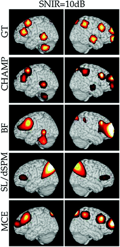
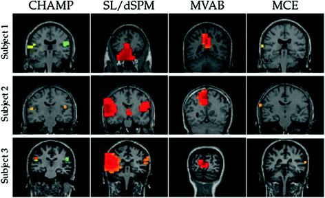

Fig. 2
Localization performance in simulations. A single example of the localization results for 10 clusters (each with 10 dipoles) at SNIR = 10 dB with the vector lead field and real brain-noise. The ground truth (GT) location of the clusters are shown for comparison, first row. The results with Champagne (CHAMP) are shown in the second row and the comparison algorithms, minimum-variance adaptive beamformer (BF), sLORETA or dSPM (SL/dSPM), and generalized minimum-current estimation (MCE) are shown in the subsequent rows. We project the source power to the surface of a template brain

Fig. 3
Auditory evoked field results for 3 subjects for four different benchmark algorithms. Champagne is able to reliably reconstruct bilateral auditory cortex activity in all subjects. SLORETA is only able to do so in two of the three subjects. MVAB fails because of the high-degree of correlations between the two sources. MCE is another sparse reconstruct algorithm that only finds auditory cortex in one hemisphere in each subject
Instead of simultaneous estimation of all sources a popular alternative is to scan the brain and estimate source amplitude at each source location independently. It can be shown that such scanning methods are closely related to whole-brain imaging methods, and the most popular scanning algorithms are adaptive spatial filtering techniques, more commonly referred to as “adaptive beamformers” or just “beamformers” (Sekihara and Nagarajan 2008). Adaptive beamformers have been shown to be quite simple to implement and are powerful techniques for characterizing cortical oscillations and are closely related to other whole-brain imaging methods. However, one major problem with adaptive beamformers is that they are extremely sensitive to the presence of strongly correlated sources. Although they are robust to moderate correlations, in the case of auditory studies, since auditory cortices are largely synchronous in their activity across the two hemisphere, these algorithms tend to perform poor for auditory evoked datasets without workarounds), and many modifications have been proposed for reducing the influence of correlated sources (Dalal et al. 2006). The simplest such workaround is to use half the sensors corresponding to each hemisphere separately, and this approach works surprisingly well for cross-hemispheric interactions. Other modifications to the original algorithms have been proposed in the literature that require some knowledge about the location of the correlated source region (Dalal et al. 2006; Quraan and Cheyne 2010). Recently, we have shown that significant improvements in performance can be achieved by modern Bayesian inference algorithms that are closely related to minimum-variance adaptative beamformers and these extensions allow for accurate reconstructions of a large number of sources from typical configurations of MEG sensors (Wipf et al. 2010; Zumer et al. 2007, 2008).
5 Temporal and Spatial Resolution of MEG Imaging
Since MEG data can be acquired at sub-millisecond time-scale, temporal resolution of MEG imaging is only limited by the sampling rate, typically ~1 kHz, and in principle, cortical oscillations can be observed up to 500 Hz. In contrast to its temporal resolution, determining the spatial resolution of MEG imaging is challenging because it is highly dependent on the reconstruction algorithm chosen, as well as a variety of factors such as signal-to-noise and interference-ratio, model formulation, forward-model accuracy, co-registration errors and accuracy of priors (Owen et al. 2012; Wipf et al. 2010). In general, it can be easily shown that the spatial resolution of MEG reconstruction is not limited by sensor spacing, because many adaptive methods can perform better than estimates based on spatial sampling criteria. For instance, while sensor spacing in many axial gradiometer systems is 2.2 cm, reconstruction accuracy can in some cases be as small as 3 mm! In general, co-registration errors alone can be on the order of 3 mm (Roberts et al. 2000). While whole-brain imaging algorithms, such as minimum-norm methods, have poor spatial resolution on the order of a few centimeters, the spatial resolution of adaptive spatial filtering methods, and more recent whole-brain reconstruction methods based on machine learning techniques, are difficult to generally compute because these estimates depend on the data and factors contributing to data quality etc. As a rule of thumb, for typical datasets, these newer methods can reconstruct tens-to-hundreds of sources about 0.5 cm apart (assuming time-frequency separation and detectability) and this can be considered an approximate spatial resolution for MEG, keeping in mind that under certain circumstances the spatial resolution can be even greater (Owen et al. 2012; Wipf et al. 2010).
A common myth, related to the spatial resolution of MEG, is its lack of sensitivity to gyral crown activity and relative insensitivity to deep sources. While it is a fact that for single spherical volume conductor models MEG sensors are insensitive to radially pointing dipoles, this does not necessarily translate to gyral sources. It has been shown that, using realistic volume conductor models (such as boundary element methods or multiple local-sphere models), some sensitivity to radial sources can be recovered, and that there is no predominant loss of sensitivity to gyral sources (Hillebrand and Barnes 2002). Furthermore, while there is a significant drop in sensitivity to deeper sources because their contributions will fall by approximately the square of the distance to the sensors, recovery of deep sources is an issue of the signal to noise ratio. In general, if high signal-to-noise ratio data are recorded, there is no inherent problem in recovery of deep sources with some of the newer Bayesian reconstruction methods. However, mid-brain sources have two additional problems. First, they may not have dipolar organization due to the architectures and second, the uncertainties in the lead-field increases for deep brain sources, thereby making them more difficult to reconstruct.
6 From Single Subject Reconstructions to Group Level Inference
While the power of MEG imaging is its ability to reconstruct the timing of activation across different frequency bands in single subjects, inferences across subjects require group level statistical analyses (Dalal et al. 2008


Stay updated, free articles. Join our Telegram channel

Full access? Get Clinical Tree


