INTRODUCTION
No single modality is all-encompassing for musculoskeletal diagnosis. Rather, each modality is like a tool in a toolbox, used to perform specific functions and solve specific diagnostic problems. For instance, while radiographs (“X-ray films”) are useful as screening tools for appendicular (extremity) fractures, magnetic resonance imaging (MRI) is a more useful tool for diagnosing meniscal tears in the knee. Used in varying combinations, the different modalities can diagnose and characterize a wide range of musculoskeletal pathology. Herein, we describe the various common modalities in clinical application and some examples of their usages.
RADIOGRAPHS
Radiographs are the predominant modality of musculoskeletal imaging (at the very least in terms of numbers of studies). In their current form, X-ray machines and scanners use electronic devices to produce and detect X-rays. The device used to detect the X-rays may in some sense be said to be similar to the detector in your digital camera, except that these detector plates are designed to detect photons from the X-ray region of the spectrum rather than photons of optical (light) wavelengths. Once formed at the detector plate, X-ray images are stored electronically on computers in a manner similar to how images are stored on your digital camera (albeit with specialized formatting). These X-ray images are then viewed with image storage, display, and editing software libraries called picture archiving and communication systems (PACS).
There is, of course, a more fundamental difference between image formation in digital photography and digital (or computed) radiography. In digital photography, optical photons emanate from the flash element of the camera, are reflected from the object being photographed, and are picked up by the detector in your camera, creating an image of the subject’s “surface.” Remember that X-rays have a shorter wavelength and higher energy than visible light, and more easily pass through tissue. X-rays thus pass through the patient to the detector plate, being only partially stopped (generally, scattered or absorbed) in the process. The resultant image is a cumulative superposition of multiple overlapping structures the X-ray photons encountered along their pathway through the patient. How does this occur? The internal anatomic structures of the patient are of varying densities, with structures of higher density (such as bones) preferentially attenuating the beam, and organs of lower density (such as the lung) allowing more photons to pass through. A transmission, or “shadow” image of the internal structure of the patient is so created by the X-ray photons passing through the patient.
Five fundamental tissue densities are defined in the human body, forming a method of scaling the brightness of the resulting images and so identifying anatomic structures. At the lowest end of the density spectrum is air, which appears on X-ray images as black or extreme dark gray regions. Next is fat tissue, also low density, showing itself as dark gray. Fluid is higher in density, and not usually seen in isolation, being paired with other soft tissue such as fat or muscle. Muscle density is still higher, usually appearing as a medium to light gray. Finally, at the (usually) highest naturally occurring density in the body is bone or calcification, appearing as light gray to white. Metal structures such as orthopedic fixation hardware for fractures and joint prostheses appear white. What is seen mainly in the final image are “edges” of objects, due to density differences between organs and other internal structures. If there is no significant density difference, adjacent structures or pathologies appear invisible or near invisible on plain radiograph as they cannot be individually distinguished with confidence and may require other modalities for visualization (Figure 1-1).
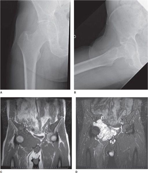
Figure 1-1. Utility of multiple imaging modalities. (A,B) Frontal and frog-leg lateral view radiographs of the right hip. (C,D) T1 and T2 fat saturation coronal MRI of pelvis demonstrating large right acetabular chondrosarcoma. The chondrosarcoma, which is easily and distinctly apparent on MRI, is more subtle on radiographs of 1A and 1B, which shows secondary bone remodeling and somewhat vague soft tissue irregularity.
Additionally, remember that the X-ray photon will pass through many structures in the patient on its way to the detector, and so many structures will be superimposed on the resulting images as a result of three-dimensional data projection into two-dimensional format. The resultant individual radiographic images are incomplete data sets (somewhat like having two equations with three unknowns), but a number of inferences and conclusions can be drawn from them. The amount of information about a particular structure (say, a joint) can be increased by taking multiple images from different perspectives. Typically, perpendicular views (frontal and lateral views) as well as an obliquely oriented view (for joints) are taken as part of a study “series.” These differing view perspectives allow objects of interest in the series to be more completely localized in space inside the patient (Figure 1-2).
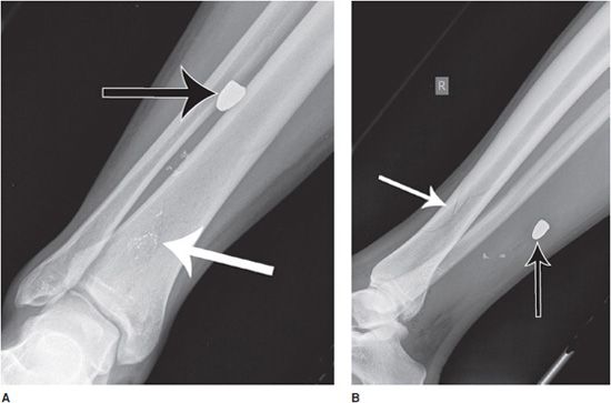
Figure 1-2. Utility of multiple image projections. Frontal (A) and lateral (B) radiograph series of the right tibia and fibula. Subtle nondisplaced comminuted fracture of the distal tibial diaphysis is apparent (white arrows). There are also multiple metallic fragments, including a bullet (black arrows). Using the frontal view (A) in isolation, it is not possible to localize the bullet any more than along an anterior-to-posterior line projection, such that the bullet may lie partially within the cortex of the tibia or fibula, or within the interosseous membrane. With the addition of the lateral projectional view, it is now possible to more completely localize the bullet location in space, projecting within the posterior soft tissues of the leg.
Radiographs are commonly used as screening examinations for fractures and joint dislocations, postsurgical follow-up of bone fixation procedures, and arthritis assessment. Drawbacks include radiation exposure for the patient, relative low sensitivity for certain types of subtle fractures such as nondisplaced intra-articular fractures, and low soft tissue contrast.1–4
COMPUTED TOMOGRAPHY
Computed tomography (CT) scanning is a sophisticated method for obtaining X-ray images of the body. As described in the radiograph section, the electronic X-ray source creates X-ray beams that penetrate and pass through multiple layers of body structure to a detector. In this case, however, the X-ray source and detectors are rotated about the patient following a cylindrical surface geometry. The beam is oriented toward the central axis of the cylinder, where the patient has been placed, while a source-detection apparatus rotates along a helical arc. Thus, the beam passes through the patient projecting from all directions (like a flashlight placed on the edge of a carousel, with the beam pointed toward the center of the carousel). A computer analyzes the degree of X-ray beam penetration through the patient at each point, and then uses sophisticated techniques to reconstruct data from these exposures and separate the objects along the beam path as it passes through the patient. The resulting volume data set is then reformatted into body “sections”—images that have the appearance of the body cut into cross sections and photographed, with each cross section viewed as an image. The computer thus creates a three-dimensional image data set from a three-dimensional structure.
Modern CT scanners can create high spatial resolution cross sections in any arbitrary plane, but typically axial, coronal, and sagittal planes (relative to the body axis in anatomic positioning) are chosen. By convention, the right side of the patient is on the left side of the computer screen while facing the screen. For axial images, it is as if you are standing at the patient’s feet looking cranially, and for coronal images, it is as if the patient is facing you.
As with radiographs, X-ray CT images represent “maps” of body organ density. These images are displayed on the PACS system in gray scale, typically with the highest density structures such as bone scaled at the bright or white end of the gray scale, and low-density material such as air at the dark or black end of the gray scale. Density units within the body as determined by the CT scanner are so scaled into units called Hounsfield units (HU) (just as units of length may be scaled as centimeters or inches). In HU, air has an approximate density of –1000 HU, fat of –100 HU, water of 0 HU, muscle of 40 HU, and bone of 1000 HU. Now, each pixel on a computer is capable of displaying a large number of intensities, or shades of gray, depending on the bit depth. For instance, 256 shades of gray are possible for 8 bits per pixel (bit depth of 8), 1024 shades at 10 bits per pixel, 4096 at 12 bits, and 65,536 at 16 bits. Most diagnostic systems are 10 or 12 bit depth. However, the human eye can only differentiate between approximately 30 shades of gray (somewhat more with training). So, only limited ranges on the gray scale (or HU scale) may thus be perceived at any time, and to appreciate this gradation, ranges of density (window width) centered about usual densities of interest (window center levels) such as bone are used to isolate and amplify anatomic details in the structures of interest.
Intravenous (IV) contrast may be used in musculoskeletal imaging studies to increase density differences between body tissues and separate adjacent structures, as well as to demonstrate physiologic processes. Except in unusual circumstances, CT examinations use iodine-based IV contrast materials due to iodine’s ability to absorb X-rays. Examples of contrast usage include delineation of the neurovascular bundles in extremities, evaluation of hyperemia in inflammatory and infectious processes, and diagnosis of hypervascular tumors. While expanding the potential usages of CT, contrast administration carries its own risks. Approximately 2% of the general population will experience a mild reaction to low-osmolar iodine contrast agents, which may include hives. Severe reactions to iodine contrast agents are seen in approximately 0.1% of the population and may include anaphylactic reactions. A summary of current symptoms, previous medical history, and medications should be obtained from the patient, with an assessment of vital signs. Treatment of milder allergic reactions (e.g., urticaria) includes observation, with possible administration of diphenhydramine. In more severe reactions, the patient should be stabilized, with monitoring of vital signs, IV fluid, epinephrine administration, and establishment of an airway, depending on clinical symptomatology. Vasovagal reactions may be treated with elevation of the patient’s legs, oxygen, IV fluid, and in more severe cases with IV atropine. Other reactions include contrast-induced nephropathy, with risk factors of contrast-induced nephropathy including elevated creatinine (<1.5 mg/dL), multiple myeloma, diabetes, and dehydration.
CT scans are commonly used for evaluating complex fractures (such as comminuted intra-articular fractures) and occult fractures (such as non- or mildly displaced intra-articular and spinal fractures), where osseous structures and fractures may be vague or obscured on radiographs (Figure 1-3). CT visualization may also be used in bone or soft tissue tumor assessment, as well as for arthrograms in cases where MRI examination is contraindicated for a particular patient. As in the case of radiographs, drawbacks again include radiation exposure (higher than a radiograph, however, progress is being made toward lower radiation doses), as well as artifact from very dense objects within (hardware) or around (external fixators, monitoring devices) the patient.4,5
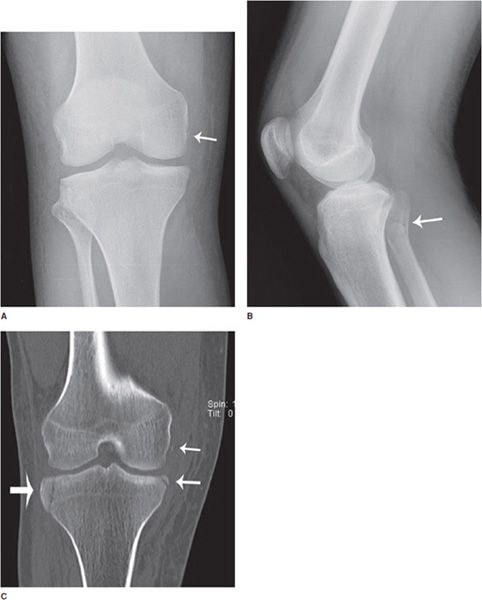
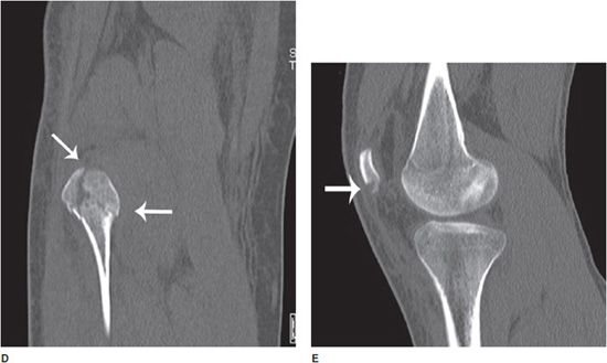
Figure 1-3. Utility of radiograph and CT. (A,B) Frontal and lateral radiographs of the right knee. There is a small cortical avulsion fracture of the medial condyle of the femur (arrow), and vaguely apparent fracturing of the fibular head (arrow). On the lateral view, joint fluid can be seen in suprapatellar bursa. (C–E) Coronal and sagittal CT images of the right knee. CT examination of bone shows fibular fracturing in more detail (arrows), as well as corner fractures of the medial and lateral tibial plateaus (arrows), and fracturing of the patella (arrow).
ULTRASOUND
Ultrasound examinations make use of the fact that sound travels with different speeds in different materials. Sound is reflected from the boundaries between anatomic structures with different compositions (which yields different internal sound speeds). Clinical ultrasound uses high-frequency sounds waves of 1–20 MHz (1 MHz is 1 million cycles per second), compared with the range of human hearing of 20 HZ-20 kHz (1 kHz is 1000 cycles per second). A probe with sound conducting material (gel) at the tip is put into contact with the body surface. The ultrasound gel is used to conduct the signal into the body tissue more efficiently, as air is a relatively poor conductor of sound waves compared with, say, water. The ultrasound probe then emits high-frequency sound waves that penetrate into the body tissues and are reflected back to the probe tip where they are detected. Using the return time and amplitude of the reflected waves, the scanner then reconstructs an image of the structures the sound waves encountered within the body. Each image typically provides a small “view portal” into the body, which sometimes gives the feeling of looking into through a tube at objects. Ultrasound is also capable of real-time visualization of the movement of structures, and so it can be used to create “cine sequences” of tendon movement, for instance. Finally, you may remember the principle of the Doppler effect from physics: sound from a source moving toward you will appear to be a higher frequency than that sound from that same source as it moves away from you. Using this principle, ultrasound may be used to measure the velocity of movement within the tissue of interest, and so it may detect and measure the velocity and direction vascular flow.
Ultrasound is a targeted modality, most commonly used in the diagnosis of pathologies in musculoskeletal structures such as tendons (rotator cuff tears and Achilles tendonitis) and for real-time guidance of musculoskeletal procedures. On the positive side, ultrasound does not involve exposing the patient to radiation, can visualize dynamic processes, and is portable. Drawbacks include relative low image resolution in many cases, limited bone penetration, and image quality dependence on the operator performing the examination.6
MAGNETIC RESONANCE IMAGING
MRI uses the magnetic properties of body tissues (in particular, the fact that different body tissues have differing magnetic properties) to create cross-sectional images of the body region of interest. Examples of body areas imaged include the knee, shoulder wrist, ankle, and hip, as well as other nonmusculoskeletal regions such as the brain. The images created are actually “maps” of the magnetic properties of the varying tissues in the body. These maps are based on nuclear magnetic resonance (NMR) spectral principles you may remember from your college organic chemistry laboratory, applied to a spatially distributed “sample,” mapping the signal at each point in space.
A simple model for the basis of MRI is that of a bar magnet, or ferromagnet, which has magnetic properties incorporating north and south poles like the earth. The magnetic poles “come out of” one side and “go into” the opposite side (by convention, north pole and south pole, respectively). This configuration is then called a magnetic dipole. So, we now know the direction of the field (out of the north pole of the magnet and back in at the south pole). If we also know how strong the field is, we can put these two quantities together to form a quantity called the magnetic moment, which then tells us the orientation and strength of the dipole. An example of a dipole you may already be familiar with is the compass, which is basically a small bar magnet (magnetic dipole). If you then put the compass into the magnetic field of the earth (another dipole), the two dipoles line up in the direction of opposite polarity (one dipole lines up in the direction of the field created by the other).
Let’s go down to the microscopic level now. The neutrons and protons that make up the nucleus of the constituent atoms and molecules of the body also have a magnetic moment. A conceptual way to think about them, then, is as miniature bar magnets in space. A simple atom that has the largest magnetic moment, and is in great abundance in the body, is hydrogen. Hydrogen is a constituent atom of a great number of molecules in the body including water (H2O), fat, and other tissues. The nucleus in hydrogen consists of a proton (like a small bar magnet). When placed in a magnetic field, the proton in hydrogen will tend to line up with it (like a compass in the earth’s magnetic field). If you were to try to turn the compass needle in the opposite direction, it would resist, and try to turn back. Therefore, you must exert energy (give energy to the compass needle) to turn the compass needle (or dipole) into the direction aligned opposite the magnetic field, which is a higher energy state.
Now, when energy is applied to the body part in the scanner in the form of an external electromagnetic field (radio wave), energy is absorbed in the tissue, putting the dipoles into a higher energy state (rotating them into the opposite direction of the field). When this external energy is removed, the dipoles relax to their lower energy state (giving off energy), but at different rates depending on the local environment (tissue type). The different relaxation rates of the dipoles in different tissues are then used to create an image.
The basic method of visualizing body tissues with MRI is to place the patient into the center of a large ring-shaped magnet, and then turn on the magnet, alternating the polarity of the magnet at various frequencies (similar to the chemical in the test tube you put into the magnet in your organic chemistry laboratory). MRI of the patient is obtained in this manner, and in the form of “sequences,” which are ways of varying MR scanner settings or parameters to emphasize different physical characteristics of tissues. While there are currently a multitude of different sequences available to scan for specific pathologies, there are a basic set of sequences seen ubiquitously in musculoskeletal (as well as other subfields of) radiology: T1, T2, and PD (proton density). Additionally, each of these sequences may be modified with a variation called “fat saturation.”
The T1 sequence is good for anatomical assessment, with a higher level of anatomic detail than seen on T2. On standard T1, fat is bright (or high signal), and generally, fluid is intermediate to dark (or low signal). However, variations do occur, with notable examples including proteinaceous fluid, which can be bright on T1 (as in the example of blood in the Met-Hb stage where it is paramagnetic), and gadolinium contrast (also a “fluid”), which is also bright on T1. With “fat saturation” (fat sat) on a T1 sequence, the fat is turned dark—now whole image appears in shades of dark gray to black (recall that fluid in generally dark on T1). Why is this important? If IV (gadolinium) contrast is given, any structure that enhances (tumor, infection, etc.) can show up as bright (light gray to white) in a background of dark gray to black (Figure 1-4).
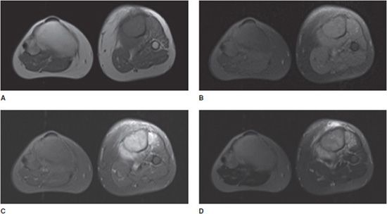
Figure 1-4. Utility of MRI for assessment of contrast enhancement. Patient with osteosarcoma of the left tibia. (A) T1 image without fat saturation. Fatty tissues appear as high signal, while muscle and fluid demonstrate intermediate signal intensity. (B) T1 image with fat saturation. Figures (A) and (B) were both obtained prior to intravenous contrast administration. Note predominant low-signal intensity on (B). (C) T1 image with fat saturation, after intravenous contrast administration. Note enhancement of the tumor in the tibia and surrounding soft tissue enhancement, as well as increased signal of lower extremity vasculature. (D) T2 fat saturation image obtained prior to intravenous contrast administration. There is increased T2 signal component within the tumor, and peritumoral edema.
The T2 sequence is useful for fluid assessment, in particular with “fat saturation” (“T2 FS”). Normally, on T2 sequences, both fat and fluid are “bright.” With “fat sat,” a signal is sent into the scanner turning fat signal intensity dark while leaving the fluid signal intensity intact (fluid stays bright). This allows better visualization of fluid in tissues. Why is this important? Fluid distinction allows for better visualization of a number of normal anatomic structures, particularly the internal structure of the joints, and edema often occurs in conjunction with tissue pathology. Pathology is usually associated with responsive edema, which helps to highlight ligament and tendon injuries, tumors, osteomyelitis, phlegmon, and abscesses, as well as acute fractures. T1 and T2 sequences may be differentiated by looking for fluid—in a joint, a cyst, or the bladder. If the fluid is bright, it is a T2 (rather than T1) sequence (Figure 1-5).
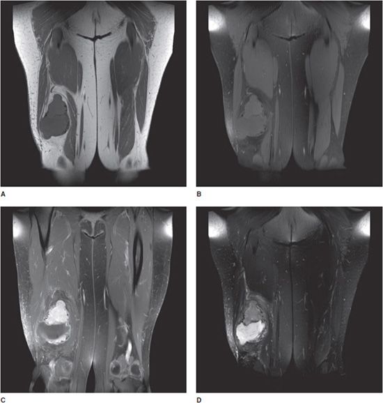
Figure 1-5. Utility of MRI for soft tissue tumor-fluid assessment. Coronal MR images of an intramuscular myxoma of the right thigh, with and without contrast. (A) T1 image without fat saturation. Subcutaneous, intermuscular, and other fatty tissues appear as high signal, with intermediate signal in muscle and fluid. (B) T1 image with fat saturation. Figures (A) and (B) were both obtained prior to intravenous contrast administration. Most structures on the fat saturation image are now low signal intensity, including subcutaneous and intermuscular fat. (C) T1 image with fat saturation, after intravenous contrast administration. Note enhancement of the vascularized tumor nidus, adjacent hyperemic tissue, and lower extremity vasculature. (D) T2 fat saturation image obtained prior to intravenous contrast administration. Fluid signal structures show high signal intensity on this T2 image, including fluid-like intensity with the tumor and adjacent reactive edema. Note tumor nidus is now of intermediate signal intensity.
The proton density (PD) sequence is intermediate between T1 and T2. On PD sequences, fluid is relatively bright and fat is bright. The PD sequence demonstrates better anatomic detail than the T2 sequence, but worse than that seen on T1. Thus, it is somewhat of a hybrid sequence between T1 and T2. So why is it of interest? Fluid is relatively bright on PD, and thus PD is good for fluid assessment, in particular with “fat saturation.” So, now we have a fluid-sensitive sequence, like T2, but with a higher level of anatomic detail available. PD is good for assessment of cartilage, among other joint structures, particularly with fat saturation (Figure 1-6).
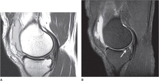
Figure 1-6. Sagittal MR images of the knee showing meniscal tear. (A) Sagittal PD without fat saturation. (B) Sagittal PD with fat saturation. Note the conspicuously bright knee joint effusion and excellent visualization of cartilage. Partially visualized linear bright signal in the meniscus reaching the articular surface of the knee representing a tear of the posterior horn of the medial meniscus (arrows).
Further extension of the above three sequences’ ability to evaluate pathology may be obtained through the administration of contrast (either IV or intra-articular, depending on the relevant pathology). In parallel to iodine-based CT contrast described above, which interacts with X-rays, contrast for MRI scans is accomplished via materials with magnetic properties. The most commonly used agents are gadolinium chelates, which are paramagnetic materials that produce magnetic moments when placed in an external magnetic foil material. As noted above, an enhancing tumor on a T1 sequence with fat saturation would show up as a region of light gray to white. Allergy to gadolinium is rare, but gadolinium should be used with caution in patients with renal failure due to the risk of nephrogenic systemic fibrosis (NSF), with the connection between the two coming to light in approximately 2006.
As in the case of CT, cross-sectional planes again demonstrate the internal anatomy of the body structure of interest. MRI is optimal for visualizing soft tissue structures of the body due to higher soft tissue contrast than CT or ultrasound, and is particularly useful for evaluating ligaments or tendons for pathology, in assessing bone infection, internal derangement of the joints, and musculoskeletal tumor evaluation. MRI does not expose the patient to ionizing radiation. A disadvantage of MRI relative to CT is the scanning time. A CT scan may now be performed in a matter of seconds, whereas for each MRI “sequence” the patient will likely have to lie motionless for 3–6 minutes. This has traditionally limited the usage of MRI for visualizing moving structures (such as bowel and heart); however, adaptive sequences have been created. Additional disadvantages of MRI include limitations of usage due to patient claustrophobia, requiring sedation or specialized visualization equipment, as well as contraindications for MR scanning such as pacemakers, neurostimulators, or cerebral aneurysm clips.4,7
MOLECULAR IMAGING (NUCLEAR MEDICINE)
In molecular imaging, molecules that preferentially localize to specific organs and regions of abnormal physiology are attached to “radiotracer” molecules. These radiotracers are usually mild- and short-lived photon or particle emitting radioisotopes, which decay and are generally excreted from the body. For instance, the half-life of the commonly used radionuclide technetium-99m (99mTc) is 6 hours; so 24 hours after the patient is injected, 6.25% of the original activity will be left. Photons emitted by the radiotracers are then absorbed by specially designed detectors, producing images either in a plane or three-dimensional cross section. Examples of detectors include gamma cameras (which detect gamma rays) and positron emission tomography (PET) scanners. Generally, gamma ray photon emitters are used as radiotracers due to the ability of gamma rays to pass through and escape body tissues, to be picked up by detectors outside the patient’s body. The detectors then create an image of the distribution of radiotracer within the patient’s body, and of particular interest, any focal abnormal radiotracer accumulation that could indicate pathology.
Thus, a benefit of molecular imaging is the integration of physiologic and anatomic information obtained from the scans. One drawback of molecular imaging scans is a spatial resolution of the resultant images, which is lower than radiographs, CT, or MRI. Other drawbacks include a requirement for specialized radiotracers and ionizing radiation exposure for patients. To overcome the spatial resolution limitation, a number of combined modality scans are now being performed, including PET/CT and single photon emission computed tomography (SPECT/CT) scans. In these cases, physiologic information from the molecular imaging scan is combined with and superimposed on high anatomic resolution CT scan (Figure 1-7). In musculoskeletal imaging, the main molecular imaging scans performed are the conventional bone scan, a three-dimensional version of bone scan called the SPECT scan, and the PET scan.
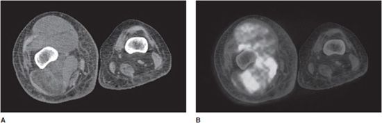
Figure 1-7. FDG PET/CT showing soft tissue mass. FDG PET/CT scan in a patient with a soft tissue tumor of the right thigh. (A) Axial CT image of the right mid-thigh. A heterogeneous soft tissue density mass is seen within the muscles of the thigh. (B) Axial co-registered (fused) image of PET/CT, same right mid-thigh region. A soft tissue density mass within the muscles of the thigh demonstrates heterogeneous increased signal intensity, corresponding to increased radiotracer uptake in regions with increased glycolysis.
BONE SCAN
In the molecular imaging bone scan, the molecule methylene diphosphonate (MDP) is attached to the radioactive tag 99mTc before injection into the patient, forming the 99mTc MDP, or “radiolabeled” MDP. The physiologic mechanism of action for this imaging agent is the binding of the MDP to hydroxyapatite crystals within the body after injection. This occurs as osteoblasts lay down (organic phase) bone matrix. Bone matrix initially consists of unmineralized osteoid with type 1 collagen and matrix proteins. Mineral deposition (inorganic phase) then occurs, with the resultant inorganic portion linked to hydroxyapatite. Accumulation of 99mTc MDP within the body is thus linked to bone turnover with associated osteoblastic activity.
So, the physiologic mechanism of action for 99mTc MDP is osteoblastic activity, which in many pathologic circumstances corresponds to focally increased bony turnover and results in focally increased 99mTc MDP accumulation. A confounding factor in this increased uptake of radiotracer to keep in mind is that uptake is also linked to increased blood flow as a mechanism of transport, and in the extreme case, no blood flow corresponds to no radiotracer uptake. Generally, however, increased uptake of 99mTc MDP is linked to increased bone turnover to a much greater extent than to increased blood flow, facilitating its usefulness for imaging. Pathologic processes can also result in focal regions of no radiotracer uptake, due to purely lytic processes (no osteoblastic activity), with examples of lytic tumors including thyroid and renal cell carcinoma metastasis.
There are two main geometries of “Bone Scan” imaging acquisition. The first is spot or planar imaging, which is the traditional method in which a bone scan is obtained (somewhat similar to a digital camera picture) with low anatomic resolution. The second is called SPECT. This is the cross-sectional version of a bone scan, similar in image geometry to a CT scan. In SPECT scanning, the three-dimensional distribution of radiotracer is imaged in a fashion somewhat analogous to the CT scan, resulting in a higher spatial resolution than the standard bone scan, but much lower resolution than a CT scan. As a side note, combined CT/SPECT is now available, where scans are performed at the same imaging session, and the computer then co-registers and superimposes SPECT images (showing regions of abnormal metabolic activity) onto CT images (for anatomy).
Increased 99mTc MDP uptake and focal accumulation in body tissues is seen in bone fracture and repair in the osteoblastic reparative process, as well as in active epiphyseal growth plates, where uptake is again related to osteoblastic activity. Increased uptake and accumulation of 99mTc MDP is also seen in conjunction with reparative processes following bone destruction due to tumors and infection. Two variants of the planar molecular imaging bone scan are commonly ordered. Whole body bone scans are usually obtained as single-phase screening scans to look at large areas of the skeleton for entities such as bone metastases (Figure 1-8). A more sophisticated study called a three-phase bone scan may be performed to rule out a bone infection, or osteomyelitis, and separate this pathology from a simple infection of the adjacent soft tissue. In the three-phase bone scan, images are obtained immediately after injection (dynamic flow phase), a few minutes after injection (blood pool phase), and 2–6 hours after injection (the static phase scan). The dynamic flow phase scan is an essential molecular imaging angiogram, showing increased or decreased blood flow to the region of interest. The blood pool phase shows soft tissue activity such as third spacing or leaky capillaries. The static phase scan is obtained to demonstrate bone involvement through osteoblastic activity, which separates sole involvement of soft tissues in the infection process (cellulitis) from combined soft tissue and underlying bone infection (cellulitis with osteomyelitis). The single-phase bone scan is performed in static phase only.
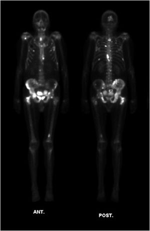
Figure 1-8. Bone scan showing bone metastases. Whole-body MDP bone scan in a patient with skeletal metastases from prostate cancer. Anterior (left) and posterior (right) images of the patient’s entire body. Note regions of expected radiotracer uptake, forming anatomic map of bones. Additionally, concentrated radiotracer in the process of excretion is noted within the bladder. There are multifocal regions of bright increased uptake corresponding to foci of bone metastasis.
PET SCAN
The most commonly used radiotracer for PET scanning is fluorine-18-fluorodeoxyglucose (18F-FDG), a glucose analog. 18F is the radiotracer in this case, emitting positrons that are annihilated as they come into contact with nearby electrons, producing two gamma rays for each collision that are then detected.
After injection, 18F-FDG becomes trapped within tumor cells. There are various theories for tumor uptake of FDG, including overexpression of glucose membrane transporter proteins in neoplastic cells and tumor hypoxia in high-grade malignancy resulting in higher rate of glycolysis. Ultimately, there is increased activity of glycolytic enzymes and glycolysis by tumor cells, which increases glucose uptake in tumor cells relative to normal cells, leading to focal increased activity on the PET scan. The FDG PET scan directly detects tumor cells, unlike the bone scan, which detects reparative activity due to tumor destruction (Figure 1-7). Uses include early lesion detection before bone scan, prediction of tumor grade in primary bone tumors, and distinguishing benign and malignant spinal compression fractures.
An alternative imaging agent for PET is fluorine-18 sodium fluoride (18F-NaF). Like the bone scan, uptake is related to osteoblastic activity (bone repair), and is taken up when fluoride ions are exchanged with hydroxyapatite crystals. 18F-NaF is reported as highly sensitive for the detection of sclerotic bone metastases (in prostate and breast cancer), among other uses8,9 (Figure 1-9).
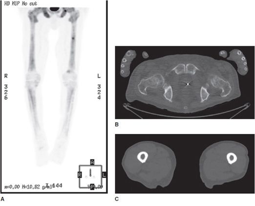
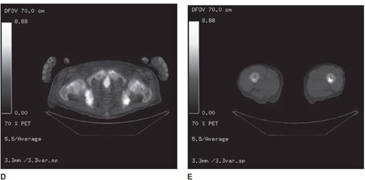
Figure 1-9. NaF PET/CT scan showing bone metastases. NaF PET/CT scan in a patient with skeletal metastasis from prostate cancer. (A) Three-dimensional PET signal reconstruction of the lower extremities demonstrating regions of expected uptake, forming visualized anatomic map of bones. Note multifocal superimposed regions of dark gray to black signal, corresponding to regions of increased uptake, and bone metastases. (B,C) Axial CT images of the pelvis and femur, respectively, with heterogeneous marrow density within the lower pelvis (prostate cancer metastases typically show as sclerotic or high density, on CT). (D,E) Same section co-registered (fused) axial PET/CT images of the pelvis and femur. Note high-signal foci in the lower pelvis image and left mid-femur corresponding to bone metastases.
Related posts:
Stay updated, free articles. Join our Telegram channel

Full access? Get Clinical Tree


