where R10 is the bulk R1 in the tissue without contrast agent. In principle, this means that a precontrast measurement of R1 should be performed before injection of the contrast agent. To convert changes in SI into changes in R1, different approaches can be used. A commonly used method is based on a phantom of tubes filled with Gd solutions at various concentrations imaged with the same sequence. The acquired SI values are plotted against measured R1 values, and a polynomial fit is made to obtain a calibration curve. However, the relaxivity is not equivalent in solution and in tissues. Another method uses the relationship between SI and R1 given by the equation driven by the sequence used (Pedersen et al. 2004), which unfortunately is not straightforward.
Other types of contrast agents have appeared in the research field with different pharmacokinetic and magnetic properties: either larger Gd-chelates or iron oxide particles (Choyke and Kobayashi 2006). The first ones do not diffuse in the interstitium, but are still filtered by the glomeruli; the second are strictly confined to the vascular space, but can be captured by activated cells with a phagocytic phenotype. If their applications remain limited today, these large molecules could be useful either for functional purposes (quantification of perfusion, quantification of GFR, estimation of tubular function) or for cellular purposes (intrarenal phagocytosis in inflammatory renal diseases).
2 Measurement of Glomerular Filtration
While the level of GFR is the best index for monitoring chronic kidney diseases (CKD), measurement of glomerular filtration is difficult to obtain accurately in routine. Therefore, the Kidney Disease Outcomes Quality Initiative (K/DOQI) of the National Kidney Foundation recommends GFR estimates for the definition, classification, and monitoring of CKD (Prigent 2008). Based on serum creatinine values, these prediction equations have limitations, especially in the normal and near-normal range of GFR, in kidney transplant recipients, and in the pediatric population. The Cockcroft and Gault formula estimates a global creatinine clearance, and the MDRD (modification of diet in renal disease study) formula estimates a GFR. The stratification of kidney diseases is based on one of these formulas in clinical practice. However, they have several limitations (Prigent 2008): variations of plasma creatinine level are around 10 %; some tubular secretion may lead to overestimation of GFR, particularly in advanced renal failure; there is a reduction of creatinine excretion with age related to a decrease in skeletal muscle mass; finally, in acute or rapidly progressing renal failure, this technique provides inaccurate information when GFR is rapidly changing.
Indications of true GFR measurements in nephrology actually include systematic follow-up of renal transplants; evaluation of living donors, when measurement of creatinine clearance is not reliable (low muscle mass, obese); and during all protocols requiring a reliable and reproducible renal function estimation.
The most common method used clinically for accurate GFR measurement is the assessment of the plasma disappearance of a substance that is excreted from the body exclusively by glomerular filtration with neither tubular reabsorption nor tubular excretion, for example, ethylenediaminetetraacetic acid (EDTA) or iothalamate (Prigent 2008). Most of the time, these standard methods are underused because they are quite time-consuming and require several blood/urinary samplings. Therefore, a quantitative method based on a tracer intrarenal kinetics, obtained rapidly, without blood and/or urine samplings, coupled with a morphological evaluation of the kidneys and the entire excretory system, would be extremely useful in the clinical management of patients with renal disease.
Besides nuclear medicine, evaluation of the filtration function is devoted to MR imaging only (Grenier et al. 2008) because US contrast agents are not filtered by the kidneys and dynamic studies require long acquisition times, making CT not acceptable in patients yet.
2.1 Measurement of Split Renal Function
Semiquantitative evaluation of renal function (RF) as split (or differential) renal function is sufficient in urological management of most uropathies, mainly obstructive. However, it is usually not useful in the daily assessment and follow-up of renal diseases. In the nephrologic field, it can be required when a reduced renal function is associated with renal asymmetry, in renovascular diseases, before renal surgery if renal function is altered or before renal biopsy. The split renal function (given in percentage) corresponds, for each kidney, to the product:
 where RFtotal is the sum of RFs of both kidneys. In clinical routine, the split renal function is still measured using nuclear medicine with glomerular (99mTc-DTPA) or tubular (99mTc-MAG3) agents. Two methods are promoted for that purpose: either the calculation of areas under the filtration curves or Rutland–Patlak plots.
Using dynamic contrast-enhanced MR imaging, Rohrschneider et al. (2000b) obtained calculations of the percentage of the single-kidney “activity” comparable to those derived with gamma camera scintigraphy. These studies were based on a dynamic RF-spoiled gradient-echo sequence and half of a standard clinical accepted dose of Gd-DTPA. A region of interest (ROI) was positioned around the renal parenchyma (omitting the pelvis), and calculation of the relative renal function was then based on the equation
 where AUC corresponds to the area under the glomerulotubular segment of the time–intensity curve and S is the ROI area (Fig. 1). In both an experimental study of ureteral obstruction (Rohrschneider et al. 2000a) and in patients (Rohrschneider et al. 2002), a high correlation between MR and renal scintigraphy was found. In addition, conversion from SI to concentration of contrast agent is not necessary as recently demonstrated in rats with acute and chronic ureteral obstruction (Pedersen et al. 2004). A large multicentric trial comparing renal scintigraphy and dynamic MR imaging in adults and children presenting with unilateral obstruction has been conducted in France (Claudon, 2014). The early results of this study show better concordance of MR estimation with renal scintigraphy using Rutland–Patlak plots than using AUC.
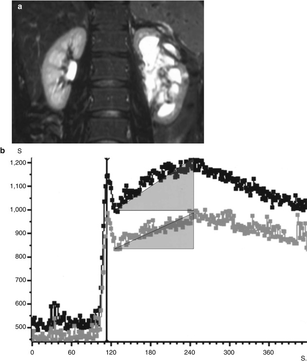
Fig. 1
Signal intensity (SI)–time curves obtained in a patient with left urinary obstruction. The anatomical image (a) shows dilatation of the left pyelocaliceal system. SI–time curves (b) obtained from regions of interest drawn on the entire renal parenchyma (excluding pyelocaliceal system) on each side, showing three phases: a first abrupt ascending segment followed by a first peak, corresponding to the “vascular-to-glomerular first pass” or cortical vascular phase; a second slowly ascending segment, ended by a second peak, corresponding to the glomerulotubular phase; and a slowly descending segment, corresponding to the predominant excretory function and the so-called excretory phase. Areas under the curves have been drawn to calculate split renal function
2.2 MR Quantification of Global GFR
Two methods are proposed for the measurement of global GFR using MRI and freely filtered Gd-chelates. The first one is based on the measurement of the clearance of an MR agent using blood samplings (Choyke et al. 1992). This method presents little advantage compared to other methods, because it is time-consuming and requires several blood samples. The second method is based on the measurement of the slope clearance of a freely filtered Gd-chelate from the extracellular fluid volume (ECFV) using SI changes within abdominal organs (Boss et al. 2007). GFR is calculated as the product of the ECFV (ECFV = 0.02154.weight0.6469 height0.3964) and the time constant of the second exponential phase (α2). The best concordance between gadobutrol clearance and iopromide clearance was observed within the liver, the exponential fit being performed between 40 and 55 min after injection (with a mean paired difference of −5.9 mL/min/1.73 m2 ± 14.6) (Fig. 2). All measurement points were within ±2 standard deviation values, but the maximum deviation from the reference GFR was 29 %. With such a wide deviation, this technique can hardly be applied to an individual patient. Main drawbacks of this method are the length of MR acquisition and the sensitivity to body movements and to the selected time intervals when the analysis is performed. More experience is required with this technique.
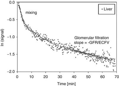
Fig. 2
Measurement of renal clearance. Exponential decay on the logarithmically scaled time–SI curve (displayed for liver parenchyma) indicates linear behavior. Two exponential phases can be distinguished owing to different slopes: the fast mixing phase immediately after contrast medium injection and the more prolonged phase, in which the SI decrease is caused solely by glomerular filtration. The negative slope of this phase is equal to the GFR divided by the ECFV (Reprinted with permission from Boss et al. 2007)
2.3 MR Quantification of Single-Kidney GFR (SKGFR)
Two methods are available for the measurement of global GFR using MRI and freely filtered Gd-chelates: (1) monitoring of tracer intrarenal kinetics and (2) measurement of the extraction fraction of the agent.
2.3.1 Monitoring of Tracer Intrarenal Kinetics
A great heterogeneity for parameters of pulse sequences, doses of injected Gd contrast, methods for the conversion of SI into concentration, postprocessing methods, and compartment models is still noted in the literature between the different groups and no consensus exists (Mendichovszky et al. 2008).
MR Technical Requirements
This quantification requires an accurate sampling of the vascular phase of the enhancement with a high temporal resolution in order to measure the arterial input function (AIF), which is characterized by the SI changes within the suprarenal abdominal aorta. It is used for the different kinetic models in order to compensate for the noninstantaneous bolus injected into the blood (Fig. 3). Not taking this into account will produce an overestimation of GFR due to recirculation of the agent within the vascular space.
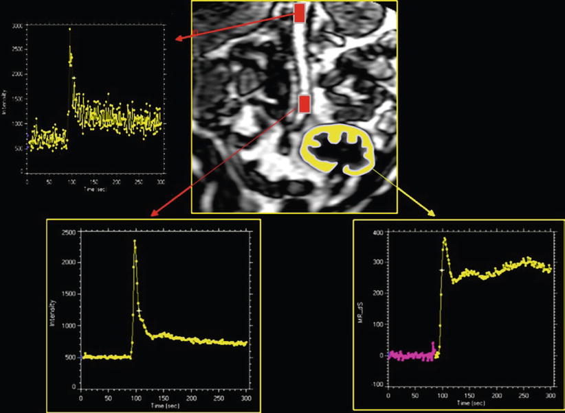
Fig. 3
Dynamic acquisition to measure GFR in a renal transplant. This requires to sample SI–time curves within aorta and within renal cortex. The aortic curve, for the characterization of the arterial input function, is altered by inflow effects only when sampling of SI is done at the top of the volume. These effects disappear in the middle of imaging plane
All pulse sequences must have a heavy T1 weighting and be fast enough to characterize the vascular phase of the tracer kinetic which is necessary for the assessment of the AIF. Therefore, sequences with a nonselective magnetization preparation are often preferred, combining with very short TR/TE and low flip angles.
Concentration of Gd within the kidney can be very high, due to water reabsorption in the proximal convoluted tubule and within the medulla. Therefore, to avoid T2* contribution to the signal, the injected dose must be lowered and the patient well hydrated (Rusinek et al. 2001). The choice between 0.025 mmol/kg and 0.05 mmol/kg depends on the level of signal-to-noise ratio obtained with the sequence and the system used.
An oblique-coronal plane, passing through the long axis of the kidneys, has to be preferred to an axial plane because, with the later, movement correction is impossible and the AIF can be severely impaired by inflow effects within the aorta.
About renal coverage, some cover the entire parenchyma with several slices using a multislice or a 3D acquisition and calculate GFR by summing the GFR values of each voxel in each slice. Others acquire only one median slice, calculate a mean GFR value, and extrapolate this value to the entire renal volume to get a total GFR.
Postprocessing
Because dynamic MRI of the kidneys is performed during free breathing, the main problem is the correction of respiratory movements. The absence of correction produces artifacts in time–intensity evolution which can lead to incorrect quantification. Gated sequences would lead to severe penalties in temporal resolution. A movement correction method developed in our group (de Senneville et al. 2008) based on the estimation of a rigid transformation and correction allowed to estimate successfully small motion and provided more than 20 % of reduction on GFR uncertainty on transplanted kidneys and up to 60 % on native kidneys (Fig. 4).
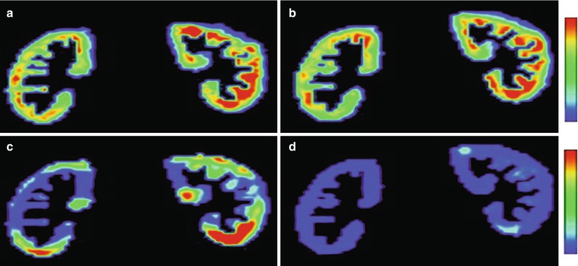
Fig. 4
Example of 2D GFR (a, b) and standard deviation (c, d) maps obtained on native kidneys without (a, c) and with (b, d) motion correction. Standard deviation values are lower and more homogeneously distributed with (d) than without (c) motion correction (Reprinted with permission from de Senneville et al. 2008)
Extraction of dynamic should be ideally limited to the cortex, which requires an accurate segmentation method. In the published clinical studies, it was generally done manually. A recent review has developed and discussed extensively the principles and the difficulties on segmentation and on renal ROI generation (Michoux et al. 2006).
Compartment Models
The ideal model reflecting filtration physiology remains to be worked out. Most of the reviewed MRI methods used a two-compartment model, although Lee et al. (2007) proposed a more complex compartment model.
The Rutland–Patlak plot technique is a graphical method based on a two-compartment model with the assumptions that the rate of change of concentration in the kidney during the clearance phase is constant if the amount of contrast agent is taken into account during this period (Patlak et al. 1983). This method has been applied to MRI by several groups (Annet et al. 2004; Hackstein et al. 2002, 2003; Hermoye et al. 2004; Pedersen et al. 2005a). The assumption that no contrast agent leaves the ROI during the sampling period may justify theoretically the use of ROIs encompassing both cortex and medulla. The model is realized as an x–y plot using the ratio of the renal concentration/aortic concentration plotted against the ratio of the integral of aortic concentration/aortic concentration. When applied to the second phase of the SI–time curve (glomerulotubular uptake), this plot leads to a straight line, with a slope proportional to the renal clearance, and an intercept with the y-axis proportional to the cortical blood volume (Fig. 5).
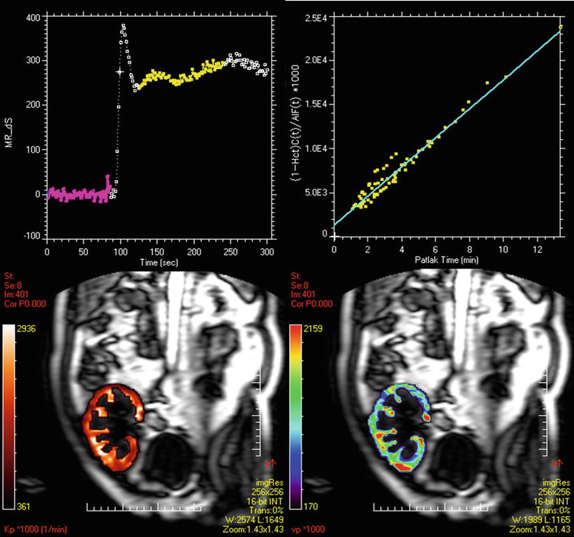
Fig. 5
Patlak–Rutland method. On the SI–time curve from the cortex of a renal transplant are selected time points corresponding to the filtration phase. The Patlak plot shows a good alignment of points. The slope corresponds to GFR. Therefore, we can draw two types of maps: the GFR map (bottom left) and the vascular volume map (bottom right)
The cortical compartment model (Annet et al. 2004; Hermoye et al. 2004) is a two-compartment model confined to the cortex, taking into account the outflow from the tubules, during the sampling period, making it possible to draw ROIs strictly limited to the cortex. Calculation of the residue function (i.e., the deconvolution of C(t) with AIF(t)) then exhibits three sequential peaks (successively glomerular, proximal tubule, distal tubule) and two rate constants, k in and k out, that describe the flow into and out of the proximal tubule, meaning that k in represents SKGFR which can be calculated according to the following equation:
To calculate C (vasc)max, the maximum of the vascular peak was divided by the renal blood volume (RBV) to take into account that the contrast agent remains in the extravascular space. This method has provided more accurate results than Rutland–Patlak model in an experimental study in rabbits, using 51Cr-EDTA as a gold standard (Annet et al. 2004). It is providing GFR, blood flow, and vascular volume (Fig. 6).
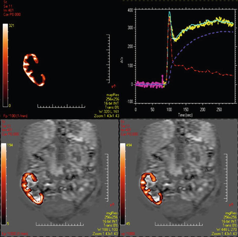
Fig. 6
Two-compartment model. From the cortical Si–time curve and from the AIF, a two-compartment model can be applied on voxel-by-voxel basis. Dynamics from each compartment can be extracted: the red curve for the perfusion component and the blue one for the filtration component. We can obtain maps of perfusion (top left) of vascular volume (bottom right) and of GFR (bottom left)
The multicompartmental model (Lee et al. 2007) includes three cortical compartments (glomerular, capillary, and proximal convoluted tubules, as in previous model), three medullary compartments (loops of Henle, distal convoluted tubules, collecting ducts), and the collecting system. Despite being complex, this model has the advantage of assessing some important tubular physiological parameters. Applied to the passage of Gd into the first two compartments, the model allows calculation of GFR.
Accuracy and Reproducibility
Such studies should be accurate and reproducible when compared to a gold standard technique. But only one clinical study undertook the 99mTc-DTPA clearance during the Gd MRI (Lee et al. 2007). A recent analysis of the literature emphasized the great heterogeneity of protocols (in acquisition mode, dose of contrast, postprocessing techniques, etc.) and regression coefficient values, which are generally considered inadequate for replacing an accepted reference method (Mendichovszky et al. 2008). While several published papers conclude that Gd-enhanced MRI provides a reliable estimate of GFR and is suitable for use in both clinical and experimental settings (Hackstein et al. 2002, 2003; Laurent et al. 2002; Lee et al. 2003), evaluation seems still necessary at a larger scale.
2.3.2 Single-Kidney Extraction Fraction
This method allows a quantification of a single-kidney (SK) extraction fraction (EF), based on the measurement of T1 within flowing arterial and venous blood (Look and Locker method) during a continuous Gd infusion (Dumoulin et al. 1994; Niendorf et al. 1996, 1997, 1998):
 where Ca and Cv are the arterial and venous Gd concentration, respectively. Because of the linear relationship between relaxation rates and concentration of Gd, EF can be expressed alternatively as:
 where T1a is T1 in the renal artery, T1v in the vein, and T10 in the blood without Gd. Once EF is calculated for each kidney, values of SKGFR can be calculated if RBF is known:
 where RBF is the renal blood flow, usually measured with the cine-phase-contrast method on the renal artery, and Hct is the level of hematocrit in the blood. Preliminary animal studies have shown concordant results with inulin clearance, but the correlation was 0.77 which is inadequate for clinical use at this stage (Fig. 3b) (Coulam et al. 2002). No clinical application of this method has been published till now.
3 Renal Flow Rate and Renal Perfusion
Renal blood flow (RBF), or flow rate, refers to the global amount of blood reaching the kidney per unit of time that is normally expressed in mL/min. This parameter is usually measured on a renal artery or a renal vein. Renal perfusion refers to the blood flow that passes through a unit mass of renal tissue (mL/min/g) in order to vascularize it and exchange with the extravascular space. The degree of perfusion depends on both the arterial flow rate and local factors such as regional blood volume and vasoreactivity. In clinical practice, measurement of RBF or perfusion may become important for the evaluation of renal artery stenosis or nephropathies with microvascular involvement and help in monitoring intravascular interventions.
3.1 Renal Flow Rate
Measurement of renal flow rate is based on the product of mean velocities in the renal artery and its section area. The cine-phase-contrast MR method is able to sample intra-arterial velocity profile and to quantify the RBF in each renal vessel without injection of contrast agent. This technique is well described in the literature (Debatin et al. 1994): it is based on the encoding of phase shifts of flowing spins either along one direction, perpendicular to the vessel of interest, or in all three directions. For accurate measurements in the human arteries, the imaging plane is usually positioned 10–15 mm downstream from the ostium, where respiratory movements are minimal, and perpendicularly to the renal artery (Fig. 7). Addition of this method to MR angiography improved interobserver and intermodality agreement as sensitivity and specificity for the detection of significant renal artery stenosis (Schoenberg et al. 1997a, b, 2002). It was also demonstrated, in vitro, that the degree of spin dephasing was directly correlated with the transstenotic pressure gradient (Mustert et al. 1998).
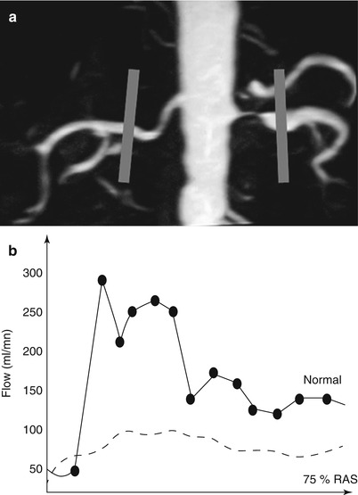
Fig. 7
Technique of cine phase contrast on renal arteries in a patient with left renal artery stenosis. Acquisition planes are positioned after each ostium, perpendicular to the arterial lumen (a). Considering the surface of the arterial lumen, velocity curves can be converted into flow rate curves. The curve from the left renal artery is damped compared to the right one (b) (Courtesy of Dr. Stephan O. Schoenberg, Heidelberg)
3.2 Renal Perfusion
3.2.1 Ultrasound
Quaia et al. (2009) applied the refilling technique to measure renal perfusion: after the blood concentration of microbubbles reached equilibrium (about 1 min after the beginning of injection), high-transmit power US pulses are sent to destroy the microbubbles filling the renal parenchyma in the imaging volume. By using a low-transmit power insonation, the progressive replenishment of the renal cortex was monitored in real time during breath-holding. A linear relation is assumed between microbubble concentration and echo–SI (Correas et al. 2000). Mathematical models previously proposed to approximate the refill kinetics of tissue after microbubble destruction present several limitations (Potdevin et al. 2004). In this study, the mathematical model used led to a piecewise linear function that has the general properties of the refill curves and took into account the laws of hydrodynamics. However, clinical applications of US-based renal perfusion studies in humans still need to be extended and validated.
3.2.2 MRI
Renal perfusion parameters, as RBV and RBF, can be assessed with MRI either by dynamic contrast-enhanced methods, using Gd-chelates or iron oxide particles, or by water spin-labeling techniques.
Dynamic MR Imaging
Technical constraints are the same as for GFR measurement. However, acquisition time is shorter, only the first pass being necessary, and breath-holding is usually efficient. If the AIF is not taken into account, semiquantitative parameters as maximal signal change (MSC), time to MSC (TMSC), or wash-in and wash-out slopes can be measured for comparison from right to left kidney (Fig. 8), from cortex to medulla or from one territory to another, or for follow-up of patients (Michaely et al. 2006, 2007a, b).

Fig. 8
Asymmetry of renal perfusion in a patient with a dissection of the left renal artery (arrow) (a). The left kidney shows irregular contours (b) and SI–time curves show a slight asymmetry of the ascending slopes and a decreased vascular peak on the left side (c)
As for GFR, absolute quantification requires to take into account the AIF. Then, the calculated concentration–time curves must then be processed using specific mathematical models (Fig. 9). The most widely used perfusion model is derived from Peters’s model (Vallee et al. 2000), developed for nuclear medicine (Peters et al. 1987). Peters et al. (1987) hypothesized that before leaving the kidney, the contrast agent behaves like microspheres that are trapped in the capillary system during a short-time interval, inferior to the minimal vascular transit time. Calculation of renal perfusion per unit of volume can be extracted from the mathematical expression
 where Δ(R1) art is calculated from the changes in aortic SI using a priori knowledge of the signal-vs.-R1 relationship that can be elucidated in vitro using a Gd-filled phantom. With a small bolus of contrast (0.025 mmol/kg) and a T1-weighted gradient-echo sequence, Vallée et al. (2000) were able to measure cortical BF in 16 normal-kidney patients (254 ± 116 mL/min/100 g), decreasing to 109 ± 75 mL/min/100 g in case of RAS and to 51 ± 34 mL/min/100 g in case of renal failure. In animals, values of cortical RBF correlated linearly with reference values, but were nonetheless systematically underestimated (Montet et al. 2003).
Fig. 9
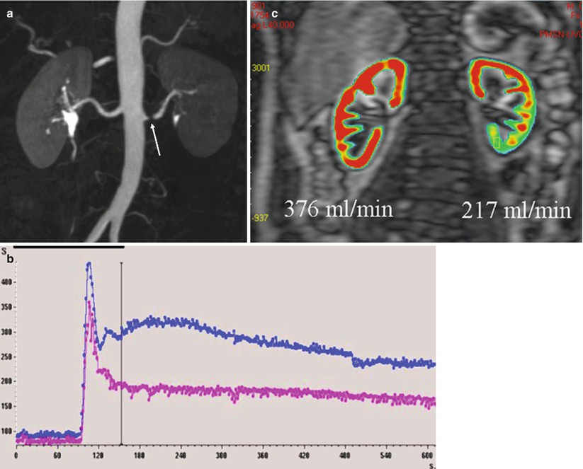
Quantification of renal perfusion in a patient with left renal artery stenosis (arrow) (a) SI–time curves show the asymmetry (b). By applying a two-compartment model and taking into account the AIF, perfusion maps can be obtained, which demonstrate the asymmetry of vascularization (c)
Dujardin et al. (2005, 2009b) generalized the tracer kinetic theory from intravascular to diffusible tracers using deconvolution, which is a model-free approach. From ROI drawn on the aorta and on the renal cortex, tissue concentration–time course has to be deconvolved pixel by pixel with the flow-corrected aortic time course, resulting in an impulse response function (IRF). This method allows getting intrarenal maps of RBF as maximum of IRF, RBV as the time integral of the IRF over the available time interval, and mean transit time (MTT) as the ratio renal volume of distribution (RVD)/RBF. They showed a significant negative correlation of RBF and RVD with patient age (Dujardin et al. 2009a).
The same approach can be applied to the measurement of perfusion using iron oxide particles which have a unicompartmental distribution within the kidney. Once injected intravenously as a bolus, they produce dynamic SI changes based on a T2* effect caused by alterations in the local magnetic susceptibility (Fig. 10). Experimental applications in rabbits subjected to hydronephrosis (Trillaud et al. 1993) or renal artery stenosis (Trillaud et al. 1995


Related posts:
Stay updated, free articles. Join our Telegram channel
Full access? Get Clinical Tree
