Computed tomography (CT) has grown quickly from an innovative specialized tool to a mainstay of medicine in every healthcare setting. Hospitals, outpatient clinics, and physician offices find CT to be an essential tool for patient diagnosis and management. Every year brings new advances in CT technology and applications. This chapter is dedicated to the basic principles and physics of CT operation. The practicing radiologist who can evaluate new technology with a good understanding of these principles will be successful in choosing the best tools for his or her practice and in getting the greatest benefit from them.
The CT Image
Radiography reduces a three-dimensional (3D) body part to a two-dimensional (2D) image with limited contrast, because structures that lie on top of one another are projected onto a single image. The contrast can be improved by using exogenous agents to enhance certain structures or by taking extra projections from different angles to separate the structures in the image plane, but there are limits to how well this can work. The advantage of CT is the improvement in image contrast that comes from using a 2D image to show an almost-2D section of the patient without the effect of overlapping structures.
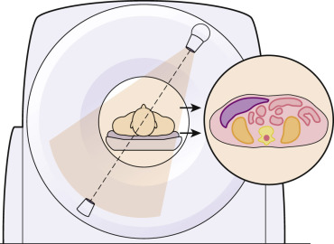
The CT image is a cross-sectional view of the patient rather than an x-ray shadow of the beam passing through the body part ( Fig. 1-1 ). An x-ray beam is used to collect information about the tissues, but the image is not an ordinary projection view from the perspective of the x-ray tube looking toward the film or detector. The image is a cross-sectional map of the x-ray attenuation of different tissues within the patient. The typical CT scan generates a transaxial image oriented in the anatomic plane of the transverse dimension of the anatomy. Reconstruction of the final image can be reformatted to provide sagittal or coronal images; these are viewed from the same perspective as a digital radiograph, but they show thin slices of tissue rather than superimposed tissues and structures. The pixel values show how strongly the tissue attenuates the scanner’s x-ray beam compared to the attenuation of the same x-ray beam by water.
The CT image is produced by the process of reconstruction: digitally combining information from x-ray projections through the patient from many different angles to produce the cross-sectional image. Because the image is digital, it is made up of a group of pixels (shortened from “picture elements”). Each pixel has a grayscale value that is displayed to the viewer. The image is 2D, but it represents a 3D volume of tissue with a finite thickness (usually a very small thickness compared to the field-of-view (FOV) size [≈2-5 mm]). Each pixel is the projection, or 2D representation, of the x-ray attenuation of a voxel (shortened from “volume element”) of physical tissue. The size of the pixels and the thickness of the voxels relate to some important image quality features, such as detail, noise, contrast, accuracy of the attenuation measurement (CT number value), and artifacts. These will be discussed in more detail as they relate to the processes of acquiring and reconstructing CT data.
CT Acquisition Overview
The basic process of collecting data in CT is illustrated in Figure 1-2 . In a CT of a single section of tissue using a single detector, the x-ray beam is collimated to the desired image thickness. The detector array has a number of individual detector elements that each record the intensity of the beam passing through the tissue along the path from the x-ray tube to the element. The system captures a simple projection x-ray through the patient, consisting of a thin strip or row of pixels. It can be thought of as a one-dimensional (1D) radiograph. The scanner then rotates the source and detector to capture additional 1D “strip x-rays” through the same section of the patient, viewed from a number of angles. Each strip radiograph (projection) is stored in the computer memory for later reconstruction.

In multislice CT ( Fig. 1-3 ) this operation is performed simultaneously for many arrays of detectors stacked side by side along the z-axis (long axis) of the patient. The x-ray beam collimators can be opened so that a wider section of the patient is irradiated, and each row of detectors can measure a separate transmission signal for the tissue section that lies between the detector row and the tube. The width of tissue that is sampled by each detector row is determined by the physical width of the detector elements along the z-axis.

CT images and individual rotations of the scanner gantry are often called slices because a single data acquisition and reconstruction produces an x-ray map of a thin section of the patient’s body. The tissue displayed in the image represents the same tissue as if a thin slice or section of the patient’s body were cut in a plane perpendicular to the long axis (superior-inferior) of the patient’s body and fixed for viewing. Early CT scanners collimated the width of the x-ray beam to the width of a slice (e.g., 5 mm), irradiated one slice at a time, and collected data for transmission through one slice at a time. Multislice scanners use a wider beam to cover more tissue with each pass of the tube, and the detectors contain arrays that are arranged to collect data for multiple individual adjacent slices at the same time. The detector element(s) for each slice store data separately and represent different physical sections of tissue.
The term slice can be confusing because in common use it can refer to several different things. When a CT scanner is called a “16-slice” model, it usually means that the scanner can acquire up to 16 individual detector data sets at one time. It is more precise to call this a 16–detector row CT scanner. The individual data elements acquired should be referred to as acquired images or acquired projection data. In a multidetector-row scanner, the data are often acquired in thicknesses of 0.5 to 0.7 mm and reconstructed in image thicknesses of 3 to 5 mm. The images that are presented to the operator or physician for viewing should be called reconstructed images, although many people continue to refer to these as slices.
Linear Attenuation and Projections
The fundamental x-ray physics of CT are the same as those for radiography. A source of ionizing radiation is transmitted through an object to recreate an image of the object based on its x-ray absorption ( Fig. 1-4 ). The intensity of the transmitted radiation beam is given by the equation:
I = I 0 e − μ x
I 0 is the incident intensity of an x-ray beam on the surface of an object of thickness x
I is the transmitted intensity
e is Euler’s constant (2.718)
µ is the linear attenuation coefficient

Attenuation of an x-ray beam with a particular spectrum depends on two distinct properties of the tissue: the atomic number and the density of the attenuating material. When collecting one projection, it is not possible to determine what combination of atomic number and density resulted in the measured attenuation. Thus both very dense materials (e.g., bone) and materials with a high atomic number (e.g., iodine contrast media) produce strong attenuation. Both would have a similar appearance on CT even though they have very different physical properties. The key advantage of dual-energy and spectral CT techniques (discussed later) is that they can be used to probe the attenuation arising from density and atomic number separately by making two different measurements of the same sample, object, or body part.
The transmission of the beam (the ratio I:I 0 ) determines the signal that is collected by the CT scanner detectors at each projection angle, and the attenuation differences along different paths through the patient’s body result in the patterns that are formed in the data for each projection acquisition.
CT Reconstruction and Image Display Overview
Once the 1D projection radiographs have been collected, they are transformed into the cross-sectional image to be displayed to the user. There are several approaches to image reconstruction, broadly classified as filtered backprojection (FBP) and iterative reconstruction (IR) techniques. All of these methods use computerized mathematical operations to combine the 1D projection attenuation information into 2D maps of the attenuation of the scanned subject.
CT Number Scale
The reconstructed CT image is a map of tissue attenuation, and these maps are quantitative owing to the use of a scale called the Hounsfield unit (HU) scale. The scale is named for the inventor of the x-ray CT scanner, Sir Godfrey Hounsfield. The HU scale is a relative scale for linear attenuation of the tissues. It is valuable to quantify the pixel values so that the physician can compare the composition of one tissue with another.
The HU scale is based on relating all measured attenuation values to the attenuation of water. A CT numbering system that relates a CT number to the linear attenuation coefficients of x-rays in different absorbers compared to water is given by:
CT Number = K ( μ − μ w ) μ w
µ w equals the attenuation coefficient of water
µ is the attenuation coefficient of the pixel in question
When K = 1000, the CT number scale is the HU scale. Other K values can be used to change the scaling of the entire system. When the HU scale is used, air has a value of −1000 HU, water has a value of 0 HU, and dense bone has a value of +1000 HU.
The advantage of the HU scale is that density differences of 1 part in 1000 (0.1%) can be represented by distinct values. The inherent density resolution of CT scanners is about 0.5%, so the HU scale is sufficient to display all attenuation differences the scanner can measure. Increasing the value of K would not improve on the density resolution of the system.
As a general rule, the human eye cannot appreciate contrast differences of less than about 10%, whereas CT scanners can easily demonstrate differences of less than 1%. Thus the small density-resolution difference measured by the CT scanner must be exaggerated for viewing. This is accomplished by enabling the user to select a small range of gray levels from the entire CT number scale and to reset the black and white limits. This is done automatically for many scanners by presetting an appropriate “window/level” setting to be used for display; this setting can be modified by the user, both on the scanner and when the image is displayed on other workstations and picture archiving and communication systems (PACS).
Generation of a CT Image
Components of a Data Acquisition System
Gantry.
Modern CT systems use slip ring technology to permit the scan frame to rotate continuously for spiral or helical CT scanning. Slip rings are used to transmit power and some control signals to the system components mounted on the gantry rotor. Systems with many detector elements and data input channels use broadband wireless communication to transmit collected image data from the detector assembly to a receiver on the stationary base of the scanner.
To enable high-speed scanning with good temporal resolution, CT system developers have focused on providing high gantry rotation speeds. For high-performance systems with mechanical roller gantry bearings, gantry rotation times of 0.33 seconds are achievable. Operating modes are available to acquire data over a partial arc (<360 degrees) to shorten the apparent rotation time further. Air bearing technology enables even faster rotation speeds. Scanners with air bearing gantry designs can achieve rotation times of 0.27 seconds. Such rotation speeds are desirable to achieve cardiac imaging without using β-blockers to slow patients’ heart rates. Together with large-coverage detector arrays, subsecond scan times permit rapid acquisition of contiguous anatomic areas for volume data acquisitions.
X-Ray Generators and Tubes.
High-frequency x-ray generators are required to produce intense x-ray beams for high-speed scanning. Typical operating frequencies range from 20 to 50 kilohertz (kHz). Generator power ratings of 80 to 120 kilowatts (kW) are common, as shown in the manufacturer specification charts for commercial systems available in the United States. Most generators support a wide range of exposure techniques from 80 to 140 kilovolts (kV) and 30 to 500 milliamperes (mA). Some generators have a lower tube potential option (70 kVp) available as an approach to radiation dose reduction. Generators are located on the rotating scan frame within the CT gantry, together with the x-ray tube and detector assembly, and are powered by a low-voltage power supply provided via the slip ring.
Modern generators have a number of features to enable them to adjust and optimize radiation output and image characteristics in real time while scanning. The generator design is computerized and flexible to allow for computer-controlled x-ray techniques generated by the scanner’s master control computer. Modulation of tube current based on patient thickness is a standard feature. Scanners may have the ability to vary the tube current along the z-axis of the patient, in the x-y plane, or both. Some systems allow dynamic or automated selection of kVp based on patient size and/or study type. For dual-energy (spectral) imaging, one approach that relies on a high-performance generator is fast kV switching. The generators for these systems can toggle rapidly (≈150 msec) between two operating voltages (usually 80 kVp and 140 kVp).
Modern CT scanner x-ray tubes have rotating anodes and use innovative cooling methods to continuous high x-ray output. Many tubes feature focal spot modulation or “flying focal spot” technology. These tubes, in addition to providing large and small focal spots, have the ability to rapidly shift the position of the selected focal spot during the scan. This has the effect of changing the sampling behavior of the scanner to enhance the resolution of the image data. Tube ratings for typical modern CT scanners can have 30 million heat units (30 MHU) of heat storage capability and a continuous output power capability of 120 kW.
Filters.
CT scanners have x-ray filters to shape both the geometry and spectrum of the beam. The standard filter is made of aluminum, like a radiographic tube filter, but there are important differences in the filter design. CT filters are generally thicker than radiographic filters and often combine other materials (e.g., Teflon, copper) with aluminum. The CT beam is much “harder” than a radiographic beam at the same kVp—it contains fewer low-energy photons and the average energy is much higher ( Fig. 1-5 ). This is done to reduce patient radiation dose (because low-energy photons are more likely to deliver dose to the patient without contributing to the image). In radiography the lower-energy photons help provide contrast to the image, but CT has much higher inherent contrast sensitivity than radiography, so a useful image can be obtained without the lower-energy photons.

The compensating filters used in CT are often called bowtie filters because of their shape. The filter is thinnest at the central ray of the beam and thicker toward the azimuthal edges of the fan beam. Thus the thinnest part of the filter is in line with the thickest path length through the patient’s body as the gantry rotates, and the thicker part of the filter is in line with the thinner peripheral anatomy (peripheral). The filter partially compensates for the patient’s body thickness contour. The result is that for any line across the FOV, the total attenuation and beam hardening along the x-ray path is much more uniform than if the beam only passed through the patient. Compensating for the attenuation differences allows the scanner to operate with a smaller dynamic range at the detectors, and compensating for the beam hardening improves the scanner’s quantitative accuracy in representing tissue attenuation as CT number values (HUs). A scanner will have at least two different bowtie filters to provide compensation for head and body scans, and some scanners have as many as five or six different filters to match a variety of patient body sizes. The bowtie filter is selected by the scanner and switched into the beam path automatically based on the scan setup chosen by the operator.
Detectors.
CT scanners use scintillation crystals to convert x-rays to visible light pulses, which in turn can be detected and counted by electronic circuits. Conventional detectors produce light pulses and voltage pulses, resulting in a simple count of x-ray photons detected. Research is underway to develop photon counting devices that can detect the number of x-ray photons as well as information about the energy of each individual photon.
CT detectors use crystals composed of fast scintillator ceramics such as cadmium telluride and gadolinium oxysulfide. Development of new crystal materials is an active area of research to further improve scanner performance, and each CT manufacturer has newer proprietary crystal types available or in development. The crystals convert x-rays to light pulses whose intensity is proportional to the total energy of photons striking the crystal. The light is converted to current and hence a voltage across a resistance, which in turn is detected as digital data for use by the reconstruction system. This multistep process of analog signal conversion to digital data produces a number of errors and inefficiencies related to quantization error, sampling and recovery speed, and electronic noise. Despite these inefficiencies, even primitive CT devices can measure low-level signals accurately over a wide dynamic range with great precision, permitting reliable imaging of diverse density extremes such as bone, air, and water.
Detector arrays continue to grow as individual detector elements remain small, providing small pixel size with ever-greater anatomic coverage. Common detector arrays accommodate scanning of 80 to 160 mm of coverage in a single tube rotation, with resolution of 0.5 to 0.6 mm, so that entire sections of patient anatomy can be captured in a single revolution of the CT scanner’s rotating frame, taking less than 1 second.
Because of the fixed position of the tube/detector combination, the associated detectors and electronics system must be stable, uniform, and capable of tracking over a wide dynamic range. Noncompensation for errors as small as a few thousandths of 1% can cause visible (ring) artifacts. In addition, spatial resolution, a key image quality parameter of CT (see later), can be limited by the data sampling. In this geometric relationship, the number of detectors in the arc or array determines data sampling; that is, spatial resolution depends on how closely spaced the rays are in each view.
The typical number of detectors in the array ranges from about 600 to more than 900. These numbers result in limiting spatial resolution of approximately 5 to 10 line pairs per centimeter (lp/cm), depending on the reconstruction type (filter), reconstruction matrix size, and scan FOV. Sampling theory requires that to visualize a particular object, the sampling frequency must be at least twice the spatial frequency associated with the object. In practice even higher sampling rates are desirable. Axial resolution of greater than 5 to 10 lp/cm (0.5-1.0 mm) may be limiting for specific clinical applications.
Data Acquisition Systems
Data acquisition systems (DAS) are the heart of CT scanners. These systems perform detector signal analog-to-digital conversion and data preprocessing for the scanner’s reconstruction system. Steps performed by the DAS include conversion of electric current (from the detector) to voltage, digitization of voltage pulses, subtraction of background offset signal, logarithmic conversion of data, and transmission of data to the preprocessing system. In modern systems, these functions are integrated and combine multiple steps on specialized hardware—boards, chips, or modules integrated into detector modules that can be housed on the detector assembly within the rotating scan frame.
An ideal DAS would accurately and consistently digitize the input signal from the detectors with no noise. The inherent electronic noise produced within the DAS must be small enough that the total noise in the sampled signal depends mostly on the x-ray quantum noise. The DAS must also have a wide dynamic range and be as linear as possible across the range of possible input signals so that the x-ray beam intensity can be accurately determined for the range of available x-ray outputs as well as a wide variety of attenuation types (tissues) and thicknesses.
A DAS will have some dark current that can vary with temperature and over time, affecting the precision (reproducibility) of the detector signal measurement. A low dark current that is stable with ambient temperature changes is desirable. Crosstalk limits the DAS performance when residual signal from one sample is collected as part of the next sample. A high-performance DAS must be capable of high sampling rates with low crosstalk.
Scanner Operation and Data Acquisition
Rotate/Rotate Scanner Geometry.
During the development of CT, several combinations of x-ray tube and detector movement were used to collect data. The historical significance of each is described in previous editions of this book. The rotate/rotate geometry emerged as the best practical design choice for high-speed scanning in multidetector-row systems and is the geometry used currently in modern multidetector CT systems.
In a rotate/rotate system the x-ray tube and detector array are mounted opposite each other on the rotating scan frame as shown in Figure 1-2 . A wide-angle fan-beam geometry (50-55 degrees) is used, and an arc of detectors and the x-ray tube rotate continuously around the patient for 360 degrees. Projection data (or data samples) are obtained at various angles, and for each angular sample taken at a position of the tube and detector, a view is created.
In rotate/rotate geometry, the detectors are fixed radially and do not view the scan area uniformly. Only the center detectors in the array “see” the pixels at the center of the FOV. However, this fixed relationship allows the detectors to be highly collimated, which greatly reduces detection of scattered radiation; this maintains contrast in the image so that the viewer will be able to detect objects against a higher background of image noise (or mottle, or grainy background).
To overcome the limitations of detector size on spatial resolution, manufacturers have developed various methods that exploit the scanner geometry. One method of increasing spatial sampling (and spatial resolution) is to offset the detector array relative to the center of rotation by a quarter-ray or eighth-ray. This allows data collected during the second half of a 360-degree rotation to be interleaved with that of the first half, effectively doubling the sampling and resolution. Patient motion can reduce this benefit. In addition, this method is limited in spiral CT scanning to certain modes in which data from projections acquired through 360 degrees are available for interleaving.
Another effective method of increasing data sampling is to oscillate the x-ray tube focal spot a few millimeters during a scan ( Fig. 1-6 ) to achieve interleaved data samples. The position of the focal spot is accurately controlled and synchronized with rotational speed and position of the rotating frame. Data acquired during the use of each focal spot position are stored separately and then interleaved to provide greater spatial sampling of the tissue. This approach can be used to increase sampling within the scan plane as shown in Figure 1-6 , and can also be used to provide increased sampling along the z-axis. When focal spot modulation is done along the z-axis, the finer sampling can be used to produce sagittal and coronal reformatted images with smaller pixel sizes than would be possible with the physical detector elements alone. Systems with this capability are often marketed as having more “slices” than the number of actual detector rows available on the scanner; for example, a scanner with 32 detector rows may be marketed as “64 slice” or a scanner with 128 detector rows may be marketed as “256 slice.”

Spatial resolution requires adequate view sampling to prevent aliasing artifacts. Views (angular projections) are limited by the electronic measurement capability of the scanner, which is typically not the gating factor for maximum resolution. These factors vary for every CT manufacturer and can dramatically affect the overall performance of a scanner.
Spiral (Helical) Scanning.
Until the late 1980s, CT scanners acquired data in discrete slices of patient anatomy in a method commonly called axial scanning. In axial (cross-sectional) CT, each revolution of the x-ray tube around the patient produces a single data set (slice). During data collection, the patient table is motionless. To create an additional slice, the table is translated by a given amount and the x-ray tube rotates around the patient again. Each rotation produces a single image. The advent of slip-ring technology and new data reconstruction techniques enabled spiral, or helical, CT.
In spiral/helical CT, the patient table translates through the gantry while the scan frame rotates continuously around the patient, sampling data as a volume. This permits new options in reconstruction. For example, once a volume of data is collected, an image can be reconstructed at any point along the effective path traced by the x-ray tube. There are several key terms associated with helical scanning:
Acquisition is the entire volume of data collected during a continuous spiral scan.
Revolution s refer to the number of 360-degree rotations of the x-ray tube during a single acquisition.
Pitch is the distance the couch travels during one 360-degree revolution of the x-ray tube divided by a length associated with the x-ray beam and/or data acquisition. The most common value used (as in the International Electrotechnical Commission [IEC] definition) is the width of the collimated fan beam along the z-axis of the scanner.
Interpolation is a reconstruction method (most accurately described as “deconvolution”) that permits the realignment of spiral/helical scan data for reconstruction of an axial (cross-sectional) slice.
Spiral CT has many advantages over conventional or axial CT, including:
- •
The ability to minimize motion artifacts owing to faster/shorter acquisitions
- •
Decreased incidence of misregistration between consecutive axial slices
- •
Reduced patient dose
- •
Improved spatial resolution in the z-axis
- •
Enhanced multiplanar or 3D renderings
Motion artifacts are minimized in spiral CT because of the faster scan times associated with the examination (versus step-and-shoot axial scanning); many spiral CT examinations can be completed in a single patient breath hold. The faster scan times associated with spiral CT also permit accurate slice-to-slice registration and eliminate the misregistration associated with inconsistent breath holds in conventional axial scanning. Reconstructions can be overlapped or ideally positioned for accurate visualization of small lesions.
Spiral scanners achieve reduced patient dose by extending the pitch factor for a given study. For example, consider a typical thorax, abdomen, or pelvis examination. Typical slice widths range from 2 to 5 mm. With spiral CT, the same examination with the same slice thickness as axial CT can be completed with 50% greater table speed using a pitch of 1.5; this results in a 33% reduction in patient dose ( Fig. 1-7 ). The downside to this approach is a slight broadening of the slice sensitivity profile (effective axial slice thickness) based on the type of spiral reconstruction chosen. This limits the spatial resolution along the z-axis, which can reduce the detail available in sagittal or coronal reformatted images.

With continuous collection of data, spiral CT enables a reduction in image-to-image separation, thus improving spatial resolution in the z-axis if the data are oversampled (pitch < 1.0). Although axial CT might overcome this challenge by overlapping consecutive axial acquisitions, this would lengthen scan time needed to cover a given region of patient anatomy more than doing so in a helical acquisition.
Spiral CT data acquisition systems must be capable of collecting large volumes of data at extremely fast data rates. Data sampling for most systems is in the range of 3 kHz and can provide up to nearly 2400 projections or views per rotation of the gantry. Data rates for many new systems exceed 200 megabits/second. This extremely fast sampling capability enables high spatial resolution and enhanced z-axis sampling of patient anatomy.
The increased speed of data acquisition systems and a number of other technologic developments paved the way for data acquisition at subsecond rotation speeds of the rotating frame. Subsecond spiral data acquisition permits temporal resolution on the order of 220 to 300 milliseconds, depending on the scanner manufacturer. These temporal resolutions enable more examinations to be scanned within a single breath hold and increase the range of anatomy that can be covered in a single acquisition. This improves the performance of clinical applications such as CT angiography, which requires precise timing of a contrast bolus injection and rapid acquisition during the arterial phase. Fast data acquisition can also improve the z-axis resolution for a given study by covering the same amount of anatomy in the same time with thinner slices and/or with oversampling at low pitch.
Multidetector-Row Designs.
Multidetector-row scanners are motivated by the desire to cover large regions of anatomy in short times with fine sampling along the z-axis of the patient. In early scanners with only a single data acquisition channel (single slice), the beam width directly determined the coverage as well as the image thickness (spatial resolution). With the development of fast, stable, compact electronics, it became possible to build a DAS that could simultaneously acquire and store multiple images. By arranging multiple narrow detector rows side by side along the z-axis, connecting them to a DAS with multiple input channels, and increasing the x-ray collimation width to cover the entire assembly, scanner designers provided users with more flexibility to achieve faster scans or finer spatial detail.
The first deployment of this technology included a dual-arc detector as shown in Figure 1-8 . In this configuration, two parallel arcs of detectors are used to acquire data simultaneously during a single revolution of the scan frame, dividing the total x-ray beam into two equal beams defined by the detector aperture of each row of detectors. Considering small gaps between rows, which can be ignored from the perspective of data acquisition, the total x-ray beam collimation now becomes the sum of detector row collimations ( Fig. 1-9 ). This concept can be extended to for systems with multiple rows of detectors.


Early multidetector-row systems were commonly equipped with a four-channel DAS. Such systems were often referred to as “four-slice” CT scanners because they could collect up to four images simultaneously in a single rotation of the scan frame. A user upgrading to such a system from a single-detector system would have the flexibility when imaging 5-mm slices to increase acquisition speed or to use finer spatial sampling in the z direction. Configuring the scanner to simultaneously acquire four 5-mm images in each rotation using a 20-mm beam collimation would reduce the acquisition time by a factor of 4. Alternatively, sampling the data using four 1.25-mm detectors and reconstructing 5-mm images would accomplish the scan in the same period of time, but the data available for sagittal and coronal reconstructions would have finer sampling and thus a smaller pixel dimension in the z direction. A possible scheme of detector configurations for such a four-channel system is shown in Figure 1-10 .

This tradeoff between coverage and z-sampling affects systems with 2 to 16 detector rows, and such systems were designed with different available combinations of physical detector element sizes, DAS input configurations, and x-ray beam collimation widths to provide clinically useful choices. Two detector designs have been deployed by CT manufacturers, unequal width and equal width, referring to the sizes of the individual detector-row elements across the z dimension of the detector array. In systems with unequal-width detector designs, the center of the detector array contains smaller detector elements that can be connected individually to the DAS for fine z-sampling with individual detector channel widths such as 0.5 mm, 0.625 mm, or 1.25 mm. The outer elements are larger and are used for wide coverage applications; in such configurations, several small center elements are electronically combined into one DAS channel. For example, one DAS channel could connect to a single outer-row element with 2.5-mm width, while another DAS channel could collect data from four 0.625 elements acting as a single 2.5-mm element. In this arrangement, the data from the four 0.625-mm elements cannot be recovered as individual z-samples, because they are combined at the input to the DAS, so the effective z-sampling is based on 2.5-mm channel widths for this scan. An alternative design is the equal-width design, where all of the detector elements have the same physical width and are connected to individual DAS channels or grouped in combination depending on the application and the needed resolution and coverage. For systems with more than 16 detector channels, it is possible for most applications to use an equal-width detector with submillimeter elements (0.5 mm or 0.625 mm are common) and provide isotropic z-sampling across the entire detector array with wide coverage. For example, a 64-detector-row system with 0.625 mm detectors can sample 40 mm of coverage with each scanner rotation while providing a separate DAS channel for each individual detector row.
Multirow detector arrays have rapidly progressed from having 2 or 4 detector rows to 64, 128, 256, and up to 320 rows in commercial CT systems. This is possible because the miniaturization of electronics enables more detector and DAS components to be installed in a detector assembly that can be practically attached to the rotating scan frame, given its size and weight. Systems with many detector rows also require advanced low-power-consumption electronics or larger power supplies to support the detector and DAS; practical limitations on these systems include providing adequate cooling for the electronics within the scanner housing. These systems use a wireless link to transfer data from the DAS on the rotating frame to the scanner’s reconstruction system, so capturing many channels of data simultaneously with high sampling rates requires a high-throughput wireless link. Advances in high-speed wireless data technology have enabled the 256- to 320-channel configurations in use in current systems, and it is possible that still larger numbers of data channels will be used the future.
CT Technique Factors
CT technique factors are the settings that are selected by the operator at the scanner’s control panel. Each has a specific effect on radiation dose to the patient and the characteristics of the scanned images. The technique factors for a scan describe the x-ray beam parameters and the geometry of the scan.
The x-ray technique factors in CT are familiar from conventional radiography. The kilovoltage (kV) applied to the x-ray tube and the tube current (mA) are selected by the operator. The exposure time is usually chosen to be the time of one complete 360-degree rotation of the rotating scan frame, so the speed of the rotation is adjusted for each scan to achieve the desired exposure time. These typically range from 0.4 to 1.0 seconds, although shorter times and faster speeds are possible.
The selection of a helical (spiral) or axial (step-and-shoot) scanning mode is a key technique factor for the scanning geometry.
The collimation of the x-ray beam along the z-axis is normally not selected directly by the operator, but rather is chosen by the scanner to match the detector configuration. Detector configuration refers to the size (length along the z-axis) of individual data acquisition channels and the total number of such channels or rows along the z-axis. For example, 64 rows of 0.625-mm detectors (N = 64, T = 0.625 mm) would be used with a total collimated beam width of 40 mm. On some systems the user may select the detailed detector configuration to achieve a certain degree of z-sampling/spatial resolution for multiplanar reconstructions. The scanner software will often choose a detector configuration automatically based on the selected reconstructed image thickness.
The pitch is a geometric technique factor in helical scanning. The coverage and scanning speed can be determined from N × T, rotation time, and pitch (for a helical scan). In this way, faster rotation speeds and wider beams covering greater z extent of the patient are used to achieve faster scans of a given anatomic region.
The scan FOV is chosen to approximately match the body size being scanned. On some scanners there are only two modes (Head and Body); other scanners have an array of SFOV size choices to contour to various patient sizes and body parts more closely.
Automatic exposure control and tube current modulation are particularly critical for radiation dose management in modern CT. These technologies usually have a few parameters and settings to control how they operate. Use of these tools and the settings used make up part of the technique factors.
Although not technically part of technique factors, reconstruction, postprocessing, and display techniques all have a dramatic impact on the quality and appearance of the images that are eventually produced.
Automatic Tube Current Selection and Modulation
In an ideal scenario, dose and image quality would be optimized by delivering the same x-ray beam flux to the detector for every projection through the patient. Of course the density and width of a patient’s body can vary greatly within a region of interest, especially when scanning an entire body region (or multiple regions). Using a single fixed mAs value does not achieve the needed optimization; some anatomy will necessarily be depicted with inadequate image quality or exposed to excess radiation in this approach.
Automated tube current modulation (ATCM) is a tool to address this challenge. Ideally ATCM can be used to optimize the scanning parameters in real time so that each patient is exposed to just enough radiation to produce a diagnostic-quality image—and no more. Automating this process should remove variation among users and the possibility of user error. The technology can be subdivided into three related techniques: automatic tube current selection, varying the tube current along the z-axis of the patient, and varying the tube current in the x-y plane around the patient.
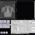
Automatic tube current selection (ATCS) is usually done by analyzing the scout/topogram image or images to estimate the attenuation of the patient and select an appropriate mAs value. The specific implementation on any given scanner may require a posteroanterior/anteroposterior (PA/AP) scout image, a lateral scout image, or both. Given the differences in patient dimension and density along a frontal versus a lateral projection, using both images should produce the most accurate choice of the correct mAs. In real implementations, most single-scout tube current modulation schemes are accurate enough.
The attenuation of the patient as measured from the scout image can be measured and expressed as the water-equivalent diameter (WED) of the patient. The WED is the diameter of a water-filled cylinder that would produce the same x-ray attenuation as the patient cross-section. This value can be very different from the physical dimension of the patient, especially in regions containing large areas of low attenuation (chest) or high attenuation (pelvis). Once the patient’s WED is determined by the scanner, the scanner chooses an mAs value based on the image quality parameter chosen by the user. In some cases this is done by specifying a target image noise value; the scanner uses calculation or lookup tables to determine what mAs value will produce the target noise for the chosen kVp and the estimated patient WED. In other cases, this is done by specifying a target or reference mAs value. In the reference mAs implementation, the reference mAs value actually represents the amount of image noise produced when a reference WED (e.g., 24 cm) is scanned with the specified mAs. Thus when a user specifies a reference mAs value of 200, what they are actually doing is asking the scanner to use an mAs value to scan the patient that will produce the same amount of noise that 200 mAs produces in the reference WED.
When using ATCS it is important to understand the specific functions as implemented by the scanner manufacturer. There are differences among commercial implementations in how the scout images are used to determine the estimated patient WED. Some scanners use the PA scout, some use the lateral, some use both, some use the first scout acquired during the examination, and some default to a fixed mAs if the expected projection (i.e., PA) is not performed first. This can lead to important workflow considerations for the technologist performing the scan. It is also important to know when designing and setting up scan protocols and technique factors on the scanner.
Z-axis tube current modulation (zTCM) is closely related to ATCS and is used to vary the tube current during each rotation of the tube, based on the different attenuation properties of different body regions. This is usually done using the estimated WED determined from the scout image. Once the baseline tube current has been established, either using automated selection or manually, zTCM is used to increase or decrease the tube current during tube rotations covering portions of the body with higher or lower attenuation. The simplest example is a scan of the chest, abdomen, and pelvis. The manually or automatically selected baseline tube current would likely be the value used to scan the abdomen, whereas a reduced current would be used in the less-dense chest and a higher current would be used to achieve good beam penetration through the dense bones in the pelvis region.
X-Y, or azimuthal, tube current modulation (aTCM) allows a further degree of fine-tuning of the radiation output to match the projection attenuation. Once the tube current is chosen to achieve a target noise level and varied based on the general density of the body region, there is still a large difference in attenuation between lateral projections and AP/PA projections. This difference is pronounced for most of the chest, abdomen, and pelvis when patients are imaged in supine or prone positions, and is especially pronounced in the shoulders and hips because of the dense bones that are superimposed in lateral projections. For scanners capable of varying the current within a single tube rotation, a modulation scheme may be available to reduce the current for AP and PA projections and increase it for lateral projections. In a variation of this approach, azimuthal modulation can be used to target exposure reduction to certain organs. For example, to reduce radiation dose to the eyes during a head scan or to the breasts during a chest scan, the azimuthal modulation can be modified to further reduce the mAs during the AP projection and compensate with increasing mAs for the lateral and/or PA projections.
In practice these three techniques may be available as separate options or activated together as part of an automated scanning mode, depending on the manufacturer’s implementation. Some manufacturers have extended this concept further by providing organ-specific boost functions (to fine-tube target noise values in specific anatomic regions) and enabling the operator to automate the selection of tube kV based on the patient attenuation determined from the scout image(s).
Dual-Energy/Spectral Acquisition
Transmission measurements in conventional CT are a physical measure of the linear attenuation properties of tissue, as described earlier. Linear attenuation depends on two underlying properties—density and atomic number—that cannot be measured separately in a single transmission measurement. However, if a sample’s transmission is measured using two different beam spectra, the two different attenuation measurements can be used to separate the two components of attenuation.
This property can be useful to probe the chemical composition of a sample. For example, a blood vessel containing iodinated contrast attenuates x-ray much more strongly than a vessel with contrast-free blood, although both have about the same density. The k-edge of iodine (determined from its atomic structure) makes it a strong attenuator. If the two vessels were imaged in a dual-energy mode and information about the physical density were recovered (independent of the atomic structure effects), the two vessels would appear to have about the same attenuation. Similarly the chemical composition of solids such as renal calculi can be probed with multiple x-ray energies to assess the content and composition of calculi having similar physical densities.
The most promising applications for dual-energy and spectral CT capabilities are virtual noncontrast (VNC) exams, iodine quantification, and calcium quantification. Dual-energy/spectral reconstructions can also prevent beam hardening artifacts and related errors in attenuation quantification (HU values).
There are several commercially available CT scanner design implementations that provide options for dual-energy or spectral CT scanning.
Dual Source
The dual source scanner employs two complete imaging assemblies, each consisting of an x-ray tube and detector array mounted at right angles to one another and aligned to scan the same plane simultaneously ( Fig. 1-11 ). This approach increases the amount of azimuthal detector coverage so that 360-degree sampling can be achieved with a partial revolution of the scanning frame; for very fast rotations, this greatly increases scanning speed. Each x-ray tube can be operated at a different kV and mAs setting, and the data from the two detector arrays can be stored separately, so it is straightforward to enable the dual-source scanner to operate in a dual-energy mode. A typical approach would be to operate one tube at 80 kV and the other tube at 140 kV.

The dual-source approach has several limitations. First, the second detector covers a smaller arc than the main detector, so the FOV is limited for any dual-source scan (whether high-speed or dual-energy). Second, the data collection for each of the two detectors is offset from the other by a quarter rotation (in space and time), so the two energy measurements are not simultaneous. There can be misregistration between the two energy images if there is patient motion during the scan.
Fast kV Switching
Scanners that use fast kV switching to provide dual-energy scanning have special x-ray generators (discussed earlier) capable of alternating the kV to the x-ray tube approximately every 150 ms so that data for the two spectra are acquired for interleaved azimuthal projections during the tube rotation. A typical acquisition would involve toggling between 80 kV and 140 kV. The data acquisition is synchronized to the kV switching so that the high- and low-energy data are stored separately to produce two different attenuation measurements in the tissue.
Fast kV switching does not provide truly simultaneous acquisition of the two spectral measurements, but there is less spatial and temporal offset than in dual source. A fast kV switching scan would thus be less prone to misregistration between the two energy scans due to motion. Fast kV switching dual-energy scanning requires that the detectors contain scintillators with very fast light decay to prevent crosstalk between the energy measurements. In current commercial systems, the x-ray generator is not able to provide tube current modulation in fast kV switching modes, so manual tube current selection must be used, forgoing some tailoring of radiation exposure to the patient.
Dual Detector
The dual detector approach uses a dual-layer detector exposed to a single x-ray beam. Because the beam has a wide energy spectrum, the top detector layer detects the low-energy photons, while the higher-energy photons pass through the top layer and are detected in the bottom layer. The detector is characterized to determine which portion of the spectrum is detected by each layer. The signals from the two layers are stored separately to provide two distinct energy-related transmission measurements.
Unlike dual source and fast kV switching approaches, there is no need to prospectively select dual-energy operation with the dual layer detector. Every scan is inherently acquired in two detector data sets. At reconstruction these data can be combined into a conventional transmission measurement or used separately to recover density and composition information. In the dual-layer detector, all of the energy measurements are simultaneous for each projection, so there is no misregistration between the spectral signals due to motion. The major drawback to the dual-layer detector approach is that there is a large overlap in the spectra to which the top and bottom layers are sensitive, which degrades the ability to decompose the acquired data into material properties and accurately quantify the atomic number and density of species in the sample.
Reconstruction
Basic Principles
Reconstruction produces an image from the digital data, representing the attenuation coefficients of the tissue voxels, provided by the data acquisition system. The acquired scan data are composed of a large number of individual ray attenuations.
Figure 1-12 shows a simplified diagram of an x-ray beam passing through successive slabs of tissue. The exit intensity from the first slab is the entrance intensity of the second slab, and so forth. To simplify this example, we assume that each of the slabs has the same thickness (L 1 = L 2 = … L n ) and the same linear attenuation coefficient µ, so that the equation for the transmitted beam passing through the n slabs is written as:
I = I 0 e − μ L
Related posts:
Stay updated, free articles. Join our Telegram channel

Full access? Get Clinical Tree


