3 TECHNIQUES IN IMAGE SEQUENCE FILTERING FOR CLINICAL ANGIOGRAPHY*
1PAR Government Systems Corporation, 1010 Prospect Street, La Jolla, CA, 92037-4146, USA
2Department of Electrical Engineering and Computer Science, Northwestern University, Evanston, Illinois 60208-3118, USA
3.1. INTRODUCTION
The assessment of coronary diseases through the evaluation of contrast imaging has been in existence for nearly a quarter century and has unquestionably aided physicians in their clinical exams. Of equal importance is a conscientious effort to reduce the risk factors of high X-ray exposure to both the patient and the medical staff. These two conflicting demands have often resulted in the degradation of image quality caused by the acquisition of radiographic images at low radiation levels. It is this noise that is treated here, since it has the greatest bearing on the tradeoff between radiation exposure and image quality. The aim of this chapter is to address this problem by first describing the process of radiation transport as a stochastic processs. Based on this description, a noise model is proposed from which a 3-D linear filter is derived to remove this noise. Its recursive counterpart is also presented here as a means of an efficient implementation. Finally, experimental results will be shown on clinical fluoroscopic images with both simulated and actual quantum mottle.
While both of these linear filters have given favorable results in terms of improving the image quality in mottled sequences, recent work in nonlinear filtering and simultaneous motion estimation and filtering may change the impetus of research in this area of clinical angiography. Some preliminary topics and results as they apply to this application will be pointed out in this chapter as well.
Historically, in digital subtraction angiography (DSA), vessels of interest were imaged by acquiring a series of X-ray images containing iodine contrast injected peripherally and subtracting them from a “mask” image of the same area obtained before opacification.79 This noninvasive angiographic technique produces images suitable for diagnostic purposes if the structures of the mask image and contrast images are registered such as those found in renal or intracranial vasculatures. In addition, relatively low frame rate (1–2 frames/sec) image acquisitions (with a corresponding increase in exposure time) are possible for noncardiac applications if patient motion is limited. This increased radiation exposure (1 mR per frame) allows for improved contrast resolution and thus greater visibility of the area of interest.
More recently, particularly in cardiac applications, interest has focused on the use of selective intraarterial contrast administration (through the use of catheters) for the assessment of coronary disorders and visualization of higher order coronary branches. In these applications, the images are of sufficient high enough quality that image subtraction is not necessary. Correspondingly, frame rates are also higher for cardiac applications (30 frames/sec) since a longer pulse width such as that used in DSA would cause motion blurring of the vessels thus reducing the spatial resolution of the image.
Typically, for these cardiac applications, 100 to 200 frames are acquired at full radiographic levels for diagnosis (about 25 μR at the input of the image intensifier) integrating to a cumulative exposure of 3.8 mR to the image intensifier for 150 frames.76 In addition, the guidance of the catheter to the coronary region requires occasional images to be acquired at fluoroscopic levels in those parts of the body where manipulation of the catheter is difficult. At these levels, quantum mottle is easily visible. Goldberg et al.,35 have also considered the use of “boosted fluoroscopy” levels (i.e., tube current between fluoroscopic levels and full radiographic levels). These images may be sufficient for the location of stenotic regions as opposed to images acquired for quantitative coronary arteriography where full radiation levels are desirable. These different radiation levels have been developed for different tasks and the decision of which level to use has always been heavily weighed by the tradeoff of image quality versus patient safety. In addition, lower doses than these conventional levels may be desirable if post-processing of the images is possible.
Though the radiation can be lowered by acquiring frames at a lower rate (same pulse width and tube current as those in 30 frames/sec applications, but using a longer separation between pulses), objectionable flickering may result due to the jerkiness of the motion.29 In addition, cardiologists often prefer a higher frame rate in order to have a sufficient number of points in the cardiac cycle, particularly near end diastole.55
A more preferable method of dosage reduction may be to vary the dosage from frame to frame. A group investigated this approach by varying the intensity between two extreme levels (0.5 and 10 mAs), allowing high X-ray intensities for periods of maximum and minimum opacification of the vessel and low X-ray intensities in between.67
Enzmann et al.23 proposed low-dose, high-frame-rate versus regular dose, low-frame-rate subtraction angiography at the same X-ray tube voltage. However, their work was with dosages in the vicinity of 200 μR (i.e., generator parameters of 75–90 kV and 300 mA at 4–7 frames per second), which is considerably higher than the range of exposures considered in this chapter. Despite this difference, they found that low-dose techniques can be successful in cases where patient motion is limited during the data acquisition process. When this case is true, low-dose fluoroscopy can generate very accurate information regarding the iodination of the arteries of interest.
The goal in low-dose fluoroscopy and low-dose angiography is to pursue this idea of continuous variability of X-ray dosage levels from frame to frame. By increasing the exposure during relevant frames and similarly by decreasing it during less relevant frames, it is possible to effectively administer X-ray dosage levels satisfactory to both the patient’s risk and image quality. Relevant frames refers to those frames where there is considerable motion, nonlinear motion, or occlusions that a post processing algorithm such as image sequence filtering which filters multiple images by using motion estimation techniques cannot handle, or considerable noise which is not created as a direct result of the exposure level (e.g., camera noise which may arise from a sudden saturation). During the less relevant frames, filtering techniques may be employed to enhance mottle-corrupted images that would naturally arise with a dosage reduction. Before these methods can be discussed, it is necessary to mathematically characterize the phenomenon of a reduced radiation exposure and to describe its effects on image quality.
It is well known that the emission of photons from an X-ray source can be described by a Poisson process.57 When the number of photons available for imaging is limited, such as in the case of low-dose fluoroscopy, quantum noise caused by the discretization of energy into photons becomes more evident. This noise manifests itself as a granularity in the image due to statistical fluctuations in the arrival of X-ray photons at the image intensifier.9 In general, this statistical fluctuation varies in both space and time and constitutes a doubly stochastic Poisson point process10,26,75 with a spatially and temporally varying intensity function. Therefore, the noise statistics may change both spatially, from pixel to pixel, and temporally, from frame to frame depending on the intensity at that particular location. This is consistent with the notion of quantum and/or signal-dependent noise.
In this chapter, the discussion will be limited to minimum mean square error (MMSE) filtering techniques. For these techniques, it is useful to describe an additive noise model

where f is the true, unknown signal, g is the observed, degraded signal and n is the signal-dependent noise term. The spatial index, r, and the temporal index, i, indicate the spatial and temporal dependency of each term.
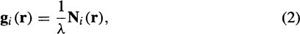
Without loss of generality, the observed degraded images are related to the observed counting processes, N, at the image intensifier through a scale factor, λ,
where Ni has a Poisson probability density function (pdf) when conditioned on the intensity f,
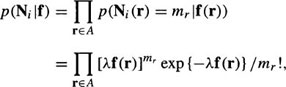
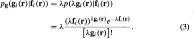
for the image plane A, as shown in Figure 1. The term, mr, represents the observed counts at pixel location r in frame i. Therefore, the displayed image intensity, g(r), has the conditional pdf
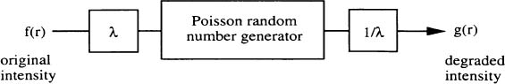
Figure 1. Poisson noise simulator, after60.
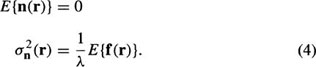
The mean and variance of the quantum noise, n(r), in Equation (1) can thus be shown to be11,54
In addition, the 3rd and 4th order moments of this noise is given by (see Appendix)
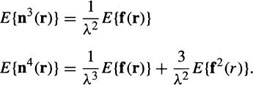
These higher order moments are useful for nonlinear MMSE filtering of images containing quantum noise,17 as this quantum noise cannot be uniquely characterized by the 1st and 2nd order moments alone as in Gaussian noise. These moments will be useful for the discussion of the nonlinear filter in Section 3.7. It can be shown,75 that the additive noise model in Equation (1) leads to an equivalent integral equation for the solution of the optimum linear estimate as that obtained if the conditional pdf in Equation (3) is used, thus justifying the formulation of such a model. Now that a model for the quantum mottle has been presented, several methods of filtering image sequences based on this model can and will be formulated in Section 3.5. First, however, a review of image sequence filtering and motion estimation is warranted.
Various filtering methods have been proposed in the past to remove noise in X-ray images. Traditionally, these methods did not assume a model for the noise and thus could not be assessed in terms of any optimality criteria other than a visual comparison.25,37 Furthermore, these methods neglect to treat the specific problem of noise arising from a reduction of radiation level (e.g., quantum mottle).
Though not specifically applied to the clinical arena, several methods for filtering single frame photon-limited scenes have been proposed in the past. Kuan et al.,54 derived a linear nonstationary minimum mean square error (MMSE) method for filtering signal-dependent noise. Poisson distributed quantum-limited noise can be seen to belong in this more general class of noise since the fluctuation of photons is directly proportional to the number of photons available in the signal (see Equation (4)). Kasturi et al.,48 through independent work, also arrived at a Bayesian estimator for treating signal-dependent noise, but taking into account the presence of additive white Gaussian noise as well in their observation equation. Jiang and Sawchuk45 expanded on Kuan’s filter by proposing to iteratively smooth a degraded image containing signal-dependent noise. Their technique also involves repeatedly updating the covariance matrix to reflect the reduction in noise levels in the image after each filtering stage. In these Bayesian techniques, different methods were used to obtain the a priori probabilities needed in the formulation of the estimators. For example, Kuan et al.,54 and Jiang and Sawchuk45 used local statistics to estimate the a priori densities of the image. This led to the nonstationary filters that they derived. Kasturi et al.,48 used a Gaussian and Laplacian model for their work. Hull et al.,42 also proposed a Bayesian approach for nuclear medicine image data, but obtained the necessary a priori probabilities from a clinical ensemble of past patient studies. Finally, Frieden27 derived a Maximum a posteriori (MAP) method for severely quantum limited images (e.g., astronomical images) wherein the noise statistics are governed by a negative binomial distribution rather than a Poisson distribution because the quantum degeneracy factor is not negligible for these types of images.
Nevertheless, given a sequence of photon-limited images, these methods would individually filter each frame independently of all other frames in the sequence without taking advantage of any temporal correlations between frames — a factor that can significantly enhance filter performance. It has been shown that simple averaging along the time axis is not an effective form of temporal processing in dynamic sequences as it tends to blur moving objects20,47 Even if these images are first registered and then averaged, the development of a model for the noise, based on physical principles, leads to a better filter, in terms of performance. Instead, the filtering of image sequences can be placed into a different class of problems.
Specifically, image sequence filtering may be classified into two categories: motion compensated and non-motion compensated. Non-motion compensated temporal filters address only the problem of estimating the intensity field by assuming that little or no motion has occurred between frames. There are two general forms of non-motion compensated temporal filters, depending on the number of filtered estimates desired. A single filtered estimate recovered from a set of observations could be obtained from a multiple-input filter, whereas simultaneous restoration of all the frames in a set of observations leading to multiple filtered estimates can be obtained through a multi-channel filter.
Ghiglia34 first addressed the problem of multiple input image restoration by considering N independently blurred images of a common object. He implemented a constrained least-squares filter in the frequency domain similar in form to the Wiener filter. Katsaggelos49 also treated this problem by using a set-theoretic approach to arrive at a least-squares solution. Hunt and Kubler43 treat the restoration of color images as a multi-channel image restoration problem. Using the MMSE criterion, they derived a multi-channel filter based on the assumption that the multispectral components can be separated through a Karhunen-Loeve transform. After this decorrelation, the images are filtered individually with a single frame Wiener filter. Galatsanos et al.,30,31 tackle the multichannel image restoration problem directly by taking into consideration cross-channel correlations without using the separability assumption and develop a multiframe Wiener restoration algorithm.
Motion compensated temporal filters, on the other hand, utilize crosscorrelations along the direction of motion. However this requires the estimation of the displacement vector field (DVF) from the noisy frames. Nevertheless, when it is available, or it can be estimated, a motion compensated temporal filter can be seen to belong in the class of multiple input filters. Huang and Tsai41 proposed one of the first techniques by doing simple averaging of the frames. For the reasons mentioned earlier, however, averaging of the frames is not an effective form of temporal processing. Dubois and Sabri20 first looked at image sequence filtering for a videoconferencing application by proposing a nonlinear recursive filter to operate on motion compensated frames. Because the motion estimator they used did not take into account the presence of noise, the results were not as good for the very noisy environments as for low noise environments. To combat this problem, Katsaggelos et al.,50 proposed a 3-D separable recursive motion-compensated spatio-temporal filter to utilize correlations not just in the temporal domain but also correlations in the spatial domain as well. The correlation coefficients were calculated for the steady state case, thus assuming that the image intensity field is stationary. To avoid this problem, an edge adaptive motion compensated spatio-temporal filter was proposed in51, where the response of the filter is tuned to spatial edge information and motion compensation prediction error. Now, however, the performance of their estimator, is also tied to the performance of the edge detector in noisy environments. Brailean and Katsaggelos5,6 have proposed a novel method for filtering image sequences in additive white Gaussian noise (AWGN) by proposing a robust motion estimator that performs well in noisy environments. In addition, an extended Kalman filter is used to filter the motion compensated image sequence. Both estimators are based on the use of doubly stochastic Markov models driven by a Gibbs distribution33 for the expression of the motion and intensity field.7
All of these image sequence filtering techniques described thus far have been formulated for sequences degraded by AWGN. Although these methods may arguably be applied to the problem at hand, they cannot correctly model the underlying quantum–limited imaging processes. For example, Singh72 used a recursive technique to perform motion-compensated enhancement of cardiac fluoroscopy image sequences. His technique follows from an incremental Kalman filtering-based method for estimating the motion field and the intensity field separately. Though he obtained good results on clinical sequences simulated with white Gaussian noise, Singh discussed the fact that X-ray images are known to have signal-dependent Poisson noise and that there is a need for temporal versions of filters for these types of noise.
3.4.2. Motion Estimation
While there have been numerous algorithms for registering angiographic images (see, for example,78,79), these methods assume that there is no noise in the images. The estimation of the DVF by specifically taking into consideration the presence of noise have only recently been considered, with the majority of the work confined to the additive white Gaussian noise (AWGN) environment. The beginnings of these works resulted primarily in maximum likelihood approaches to estimate the motion field whereby Gaussian assumptions are made to make the problem more tractable.58,61,64 Anderson and Giannakis2 considered the use of higher order cumulants for estimating the DVF in correlated Gaussian noise. Abdelqader and Rajala1 took into consideration a priori knowledge of the motion field by using Gibbs distribution and applying a mean field annealing technique to noisy sequences in order to obtain the result. Konrad and Dubois53 also used a Gibbs distribution in their characterization of the DVF, but solved for the solution using MAP and minimum expected cost methods. Brailean and Katsaggelos7 treated the problem recursively and obtained MAP estimates of the motion field from noisy sequences using an extended Kalman filter.
These approaches preclude those techniques which treat the motion field as an observed noisy signal requiring post-processing. In the application to quantum-limited scenes, Pohlig70 investigated the detection of moving optical targets from a CCD sensor in Poisson noise, but does not consider the estimation problem. Though Chen18 extends this detection problem further to account for three-dimensional moving targets, the estimation of the DVF by specifically taking into consideration the presence of noise have only recently been considered, with the majority of the work confined to the additive white Gaussian noise environment. Morris62 describes a method for scene matching using photon-limited images, but assumes the availability of an original reference scene for cross-correlation against the degraded frame. In general, the two frames of a dynamic sequence, such as those considered here, are both degraded and the original reference frame is not available. Chan and Katsaggelos16 have proposed an iterative method for estimating DVF’s from quantum-limited scenes. This approach will be described in Section 3.8. In addition, Chan et al.,8,15 extend this method further by considering the use of a Gibbs distribution to describe the motion field to improve upon the estimates.
In general, the registration of images in noise through motion compensation is a difficult problem. Consequently, in order for image sequence filtering to be optimal, the two tasks of displacement field estimation and image enhancement should be treated simultaneously as was done in15,16. In the first part of this chapter, image sequence filtering in quantum-limited noise is treated as a two-stage problem instead; that is, the estimation of the displacement field is treated separately from the estimation of the image intensity field. Although this may not provide the best possible results, separability enables a simpler, yet more insightful, formulation of the problem, while still yielding improved estimates over spatial filtering alone. Later, in Section 3.8, some preliminary work on the simultaneous motion estimation and filtering approach will be presented for the quantum-limited case.
Perfect registration of two frames, f1 and f2, undergoing purely translational motion implies that  , where d is the spatially and temporally varying DVF. The commonly made assumptions of constant brightness and no occlusions of moving objects are made here. In practice, f1 and f2 are not available for motion compensation. Therefore, the degraded observations, g1 and g2, must be used to obtain the motion vector estimates. Such an implementation is shown in Figure 2. Katsaggelos et al.50 have shown that with noise above a certain level, registration errors become so large that it is necessary to spatially filter each frame separately before motion estimation can be performed. This is also true for the clinical fluoroscopic image sequences shown in this chapter. This optional step is also shown in Figure 2.
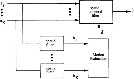
Figure 2. Block diagram of motion-compensated temporal filter.
It is important to note that displacement estimates obtained with this spatial filtering preprocessing stage are used for the temporal filtering of the degraded frames, and not the spatially filtered frames. The latter procedure of applying the temporal filter to the spatially filtered frames may result in the oversmoothing of the image causing edges to become blurred. This “iterative” filtering (so named because of applying filtering to the degraded images and then to the newly filtered image again) was implemented with Kuan’s spatial filter, as mentioned earlier, in45. It entails updating the noise covariance matrix in the original formulation to reflect the presence of new noise levels after spatial filtering once. While this approach is not addressed here, an application of a temporal version of this “iterative” filter to angiographic image sequences can be found in14.
Next, a method is described for obtaining an estimate of the vector field, d, between g1 and g2, or their spatially filtered counterparts, h1 and h2. Two different approaches have been implemented in this study — namely, a block matching algorithm using an exhaustive mean square matching criterion65 and a Wiener-based pel-recursive algorithm4,21,22 with similar filtering results. Block matching algorithms constitute shifting image subblocks between two frames to find the direction of maximum correlation. Pel (or pixel) recursive algorithms recursively compute a displacement vector for each pixel using gradient-based minimization.65 Generally, block matching algorithms are more robust to large displacements in the sequence, although the DVF produces noticeably more blocking artifacts, when used for compensation of the motion. However, this problem can be compensated for by choosing overlapping blocks and interpolating the vectors away from the center of the block. Because the fluoroscopic sequence used in the simulations may contain displacements of as much as 10 pixels between two consecutive frames, the block matching algorithm described above was used to obtain the DVF. For even larger displacements, a bigger search space may be used in the block matching algorithm. Alternatively, the radiation dosage may be raised at this point in anticipation of the jump in motion, in essence, turning off the temporal filter. Some a priori information must be utilized regarding the structure being imaged to determine whether the displacement is beyond the specifications of the motion estimation algorithm.
In the next section, a 3-D locally linear minimum mean square error (LLMMSE) filter is derived based on the noise model discussed in Section 3.3. This filter will operate on a set of registered images obtained through the motion estimation algorithm just discussed.
The proposed 3-D linear minimum mean square error (LMMSE) filter is derived in this section for the multiple-input case, which assumes the availability of a set of motion compensated frames degraded by quantum-limited noise. As discussed in the previous section, this set of registered frames is obtained separately by using a DVF which was obtained independently.
3.5.1. Filter Formulation
Consider the lexicographically ordered representation of the set of observation equations given by


∀r = 1,…, M2 and ∀i = 1,…, K – 1, where di,K (r) is the spatially varying displacement vector relating the intensity in frame i to frame K at spatial location r. Furthermore, let the motion compensated frames representing the observation and noise images be denoted by
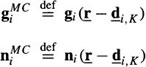
and the motion compensated original image by

Consequently, Equation (6) may be rewritten as

and

For ease of notation, these vectors are further stacked into a single observation equation resulting in

where

and similarly for f and n. All the vectors, g, f, and n, are of dimensions K M2 × 1.
Using the additive signal-dependent noise model derived in Section 3.3, a minimum mean square error estimate is sought which minimizes the mean square prediction error,

The optimal estimate,  , is given by the conditional mean66
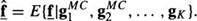
In general, this conditional mean is nonlinear. However, it was pointed out in Section 3.3 and shown in75 that the use of an additive noise model leads to an equivalent integral equation for the solution of the optimum linear estimate as that obtained if the conditional mean was constrained to be linear. In other words, the formulation of an additive noise model from the Poisson data allows one to approximate the conditional mean with a linear estimator of the form

where 1 is a vector of K M2 1’s, and the Γi’s are matrices of dimensions K M2 by M2 containing the unknown coefficients to be determined. The optimal linear estimate is given by the multichannel LMMSE filter

which is similar to the single-channel LMMSE estimator54,66, where  is the cross-covariance matrix and
  is the covariance matrix. It should be noted that this filter is different from the multichannel Wiener filter in43,30, because of the nonstationarity involved. For example, the matrix
  is not block circulant and therefore fast Fourier transform (FFT) techniques cannot be used to obtain its inverse, and all operations are performed in the spatial domain.
Because the f vector consists of K identically stacked versions of f, Equation (9) is simplified to a multiple-input LMMSE filter

where 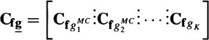 . Expanding the terms, Equation (10) becomes
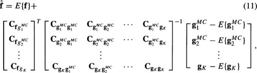
where all the submatrices are diagonal, thus making  a sub-block diagonal matrix. The similarity between this multiple-input filter and the multichannel filter in Equation (9) is evident because f1, f2, …, fK–1 are all related to fK through the respective DVF’s. In this instance, the solution for all the motion-compensated channels of the multichannel filter is identical to the solution for a single channel, as given by the multiple-input filter.
In Equation (11), the inversion of  , of dimensions K M2 × K M2, is required. Even for moderate size images, (M = 256), this inversion is unmanageable. However, the matrix is sub-block diagonal due to the nonstationary mean nonstationary variance (NMNV) assumption of no correlation between pixels, and therefore, it is a straightforward task to perform the inversion. It can be shown that the inverse has the same sub-block diagonal form and that the inversion of this K M2 by K M2 sub-block diagonal matrix can be decomposed into M2 inversions of K by K matrices.31 In other words, there exist M2 locally linear MMSE (LLMMSE) separate filters, one for each pixel. This seems reasonable, since the intensity of f is actually a mixture of Gaussians, with nonstationary means and nonstationary variances.
The term local refers to the neighborhood around the working pixel in which the spatially varying means and variances of the NMNV model are estimated. Specifically, since the means and variances vary from pixel to pixel and the pixels are jointly independent, each filter at a spatial location r operates independently of the filters at other spatial locations. Furthermore, the estimation of these nonstationary first and second order moments is also done locally — within a local spatial analysis window. A larger window can give a more accurate estimate of these statistics provided that there are no edges in the window. The presence of discontinuities can cause undesirable biases in these estimates. With motion-compensated image sequences, however, there exists K realizations of the random field. Therefore, the spatial dimensions of these local windows can be made smaller than their counterparts in the still frame case, while still providing good estimates since multiple frames are used, and the temporal dimension of these windows is greater than one.
With the above assumptions, the LLMMSE filter takes the following form at each pixel11:
where  are the local variances, and
  and
and  represent the corresponding local means of f(r) and g(r). It is interesting to note that when K = 1, the filter in Equation (12) is similar to the spatial filter for single images developed by Kuan et al. in54. For the single-frame case, the local cross-covariance,
  , can be shown to be equal to the local variance of f(r), or
  . Then, the inversion of each K by K
Related posts:
Stay updated, free articles. Join our Telegram channel

Full access? Get Clinical Tree


