Intensity-Modulated Radiation Therapy

20.1. Introduction

In the traditional external beam photon radiation therapy, most treatments are delivered with radiation beams that are of uniform intensity across the field (within the flatness specification limits). Occasionally, wedges or compensators are used to modify the intensity profile to offset contour irregularities and/or produce more uniform composite dose distributions such as in techniques using wedges. This process of changing beam intensity profiles to meet the goals of a composite plan is called intensity modulation. Thus, the compensators and wedges may be called intensity modulators, albeit much simpler than the modern computer-controlled intensity modulation systems such as dynamic multileaf collimators.

The term intensity-modulated radiation therapy (IMRT) refers to a radiation therapy technique in which nonuniform fluence is delivered to the patient from any given position of the treatment beam to optimize the composite dose distribution. The treatment criteria for plan optimization are specified by the planner and the optimal fluence profiles for a given set of beam directions are determined through “inverse planning.” The fluence files thus generated are electronically transmitted to the linear accelerator, which is computer controlled, that is, equipped with the required software and hardware to deliver the intensity-modulated beams (IMBs) as calculated.

The clinical implementation of IMRT requires at least two systems: (a) a treatment-planning computer system that can calculate nonuniform fluence maps for multiple beams directed from different directions to maximize dose to the target volume while minimizing dose to the critical normal structures, and (b) a system of delivering the nonuniform fluences as planned. Each of these systems must be appropriately tested and commissioned before actual clinical use.

20.2. Intensity-Modulated Radiation Therapy Planning

The principle of IMRT is to treat a patient from a number of different directions (or continuous arcs) with beams of nonuniform fluences, which have been optimized to deliver a high dose to the target volume and an acceptably low dose to the surrounding normal structures. The treatment-planning program divides each beam into a large number of beamlets and determines optimum setting of their fluences or weights. The optimization process involves inverse planning in which beamlet weights or intensities are adjusted to satisfy predefined dose distribution criteria for the composite plan.

A number of computer methods have been devised to calculate optimum intensity profiles (1,2,3,4,5,6,7,8,9,10). These methods, which are based on inverse planning, can be divided into two broad categories:

Analytic methods. These involve mathematical techniques in which the desired dose distribution is inverted by using a back projection algorithm. In effect, this is a reverse of a computed tomography (CT) reconstruction algorithm in which two-dimensional images are reconstructed from one-dimensional intensity functions. If one assumes that the dose distribution is the result of convolutions of a point-dose kernel and kernel density, then the reverse is also possible, namely by deconvolving a dose kernel from the desired dose distribution, one can obtain kernel
density or fluence distribution in the patient. These fluences can then be projected onto the beam geometry to create incident beam intensity profiles.

One problem with analytical methods is that, unlike CT reconstruction, exact analytical solutions do not exist for determining incident fluences that would produce the desired dose distribution without allowing negative beam weights. The problem can be circumvented by setting negative weights to zero but not without penalty in terms of unwanted deviations from the desired goal. So some algorithms have been devised to involve both analytical and iterative procedures.
Iterative methods. Optimization techniques have been devised in which beamlet weights for a given number of beams are iteratively adjusted to minimize the value of a cost function, which quantitatively represents deviation from the desired goal. For example, the cost function may be a least square function of the form:

where C_n is the cost at the nth iteration, D_o(

) is the desired dose at some point (

) in the patient, D_n(

) is the computed dose at the same point, W(

) is the weight (relative importance) factor in terms of contribution to the cost from different structures, and the sum is taken over a large N number of dose points. Thus, for targets the cost is the root mean squared difference between the desired (prescribed) dose and the realized dose. For the designated critical normal structures, the cost is the root mean squared difference between zero dose (or an acceptable low dose value) and the realized dose. The overall cost is the sum of the costs for the targets and the normal structures, based on their respective weights.

The optimization algorithm attempts to minimize the overall cost at each iteration until the desired goal (close to a predefined dose distribution) is achieved. A quadratic cost function such as that given by Equation 20.1 has only one minimum. However, when optimizing beam weights for all the beams from different directions to reach a global minimum, the same cost function exhibits multiple local minima. Therefore, in the iteration process occasionally it is necessary to accept a higher cost to avoid “trapping” in local minima. An optimization process, called simulated annealing (3,10), has been devised that allows the system to accept some higher costs in pursuit of a global minimum.

Simulated annealing takes its name from the process by which metals are annealed. The annealing process for metals involves a controlled process of slow cooling to avoid amorphous states, which can develop if the temperature is allowed to decrease too fast. In the analogous process of simulated annealing, the decision to accept a change in cost is controlled by a probability function. In other words, If ΔC_n <0, the change in the variables is always accepted. But if ΔC_n <0, the change is accepted with an acceptance probability, P_acc, given by:

where ΔC_n = C_n – C_n –C_n-1, κT_n is analogous to thermal energy at iteration n (it has the same dimensions as ΔC_n), T_n may be thought of as temperature, and κ as Boltzmann constant.¹ At the start of simulated annealing, the “thermal energy” is large, resulting in a larger probability of accepting a change in variables that gives rise to a higher cost. As the optimization process proceeds, the acceptance probability decreases exponentially in accordance with Equation 20.2 and thus drives the system to an optimal solution. The process is described by Web (10) as being analogous to a skier descending from a hilltop to the lowest point in a valley.

The patient input data for the inverse planning algorithm is the same as that needed for forward planning, as discussed in Chapter 19. Three-dimensional image data, image registration, and segmentation are all required when planning for IMRT. For each target (planning target volume [PTV]), the user enters the plan criteria: maximum dose, minimum dose, and a dose volume histogram. For the critical structures, the program requires the desired limiting dose and a dose volume histogram. Depending on the IMRT software, the user may be required to provide other data such as beam energy, beam directions, number of iterations, etc., before proceeding to optimizing intensity profiles and calculating the resulting dose distribution. The evaluation of an IMRT treatment plan also requires the same considerations as the “conventional” three-dimensional conventional radiotherapy (3-D CRT) plans, namely viewing isodose curves in orthogonal planes, individual slices, or 3-D volume surfaces. The isodose distributions are usually supplemented by dose volume histograms.

After an acceptable IMRT plan has been generated, the intensity profiles (or fluence maps) for each beam are electronically transmitted to the treatment accelerator fitted with appropriate hardware and software to deliver the planned intensity-modulated beams. The treatment-planning and
delivery systems must be integrated to ensure accurate and efficient delivery of the planned treatment. Because of the “black box” nature of the entire process, rigorous verification and quality assurance procedures are required to implement IMRT.

20.3. Intensity-Modulated Radiation Therapy Delivery

Radiation therapy accelerators normally generate x-ray beams that are flattened (made uniform by the use of flattening filters) and collimated by four moveable jaws to produce rectangular fields. Precollimation dose rate can be changed uniformly within the beam but not spatially, although the scanning beam accelerators (e.g., Microtron) have the capability of modulating the intensity of elementary scanning beams. To produce intensity-modulated fluence profiles, precalculated by a treatment plan, the accelerator must be equipped with a system that can change the given beam profile into a profile of arbitrary shape.

Many classes of intensity-modulated systems have been devised. These include compensators, wedges, transmission blocks, dynamic jaws, moving bar, multileaf collimators, tomotherapy collimators, and scanned elementary beams of variable intensity. Of these, only the last five allow dynamic intensity modulation. Compensators, wedges, and transmission blocks are manual techniques that are time consuming, are inefficient, and do not belong to the modern class of IMRT systems. Dynamic jaws are suited for creating wedge-shaped distributions but are not significantly superior to conventional metal wedges. Although a scanning beam accelerator can deliver intensity-modulated elementary beams (11), the Gaussian half-width of the photon “pencil” at the isocenter can be as large as 4 cm and therefore does not have the desired resolution by itself for full-intensity modulation. However, scanning beam may be used together with a dynamic multileaf collimator (MLC) to overcome this problem and provide an additional degree of freedom for full dynamic intensity modulation. The case of dynamic MLC with upstream fluence modulation is a powerful but complex technique that is currently possible only with scanning beam accelerators such as Microtrons (12).

For linear accelerators it seems that the computer-controlled MLC is the most practical device for delivering IMBs. Competing with this technology are the tomotherapy-based collimators—one embodied by the multileaf intensity-modulating collimator (MIMiC) collimator of the NOMOS Corporation and the other designed for a tomotherapy machine under construction at the University of Wisconsin.

A. Multileaf Collimator as Intensity Modulator

A computer-controlled multileaf collimator is not only useful in shaping beam apertures for conventional radiotherapy, but it can also be programmed to deliver IMRT. This has been done in three different ways.

A.1. Multisegmented Static Fields Delivery

The patient is treated by multiple fields and each field is subdivided into a set of subfields irradiated with uniform beam intensity levels. The subfields are created by the MLC and delivered in a stack arrangement one at a time in sequence without operator intervention. The accelerator is turned off while the leaves move to create the next subfield. The composite of dose increments delivered to each subfield creates the intensity-modulated beam as planned by the treatment-planning system. This method of IMRT delivery is also called “step-and-shoot” or “stop-and-shoot.” The theory of creating subfields and a leaf-setting sequence to generate the desired intensity modulation has been discussed by Bortfeld et al. (13). The method is illustrated in Figure 20.1 for one-dimensional intensity modulation in which a leaf pair takes up a number of static locations and the radiation from each static field thus defined is delivered at discrete intervals of fluence (shown by dotted lines). In this example ten separate fields have been stacked in a leaf-setting arrangement known as the “close-in” technique (Fig. 20.2A). Another arrangement called the “leaf sweep” is also shown (Fig. 20.2B). The two arrangements are equivalent and take the same number of cumulative monitor units. In fact, if N is the number of subfields stacked, it has been shown that there are (N!)² possible equivalent arrangements (14). The two-dimensional intensity modulation is realized as a combination of multiple subfields of different sizes and shapes created by the entire MLC.

The advantage of the step-and-shoot method is the ease of implementation from the engineering and safety points of view. A possible disadvantage is the instability of some accelerators when the beam is switched “off” (to reset the leaves) and “on” within a fraction of a second. The use of a gridded pentode gun could overcome this problem as it allows monitoring and termination of dose within about one-hundredth of a monitor unit (MU). However, not all manufacturers have this type of electron gun on their linear accelerators.

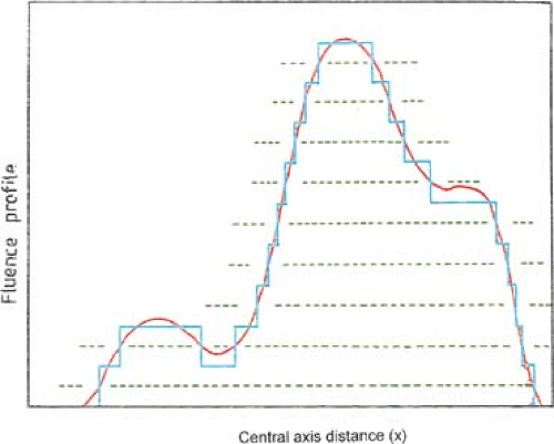Figure 20.1. Generation of one-dimensional intensity modulation profile. All left leaf settings occur at positions where the fluence is increasing and all right leaf settings occur where the fluence is decreasing. (From Web S. The Physics of Conformal Radiotherapy. Bristol, UK: Institute of Physics Publishing; 1997:131, with permission.)

A mixed mode of IMB delivery, called “dynamic-step-and-shoot,” has also been used. In this method the radiation is “on” all the time, even when the leaves are moving from one static subfield position to the next. This technique has the advantage of blurring the incremental steps in the delivery of static subfields (15).

Bortfeld et al. (13) have demonstrated that a relatively small number of steps (10–30 to cover a 20-cm wide field) can be used to deliver an intensity-modulated profile with an accuracy of 2% to 5%. A nine-field plan could be delivered in less than 20 minutes, including extra time allowed for gantry rotation (13). Figure 20.3 is an example of an intensity-modulated fluence profile generated by the step-and-shoot method and compared with calculated and measured dose.

A.2. Dynamic Delivery

In this technique the corresponding (opposing) leaves sweep simultaneously and unidirectionally, each with a different velocity as a function of time. The period that the aperture between leaves
remains open (dwell time) allows the delivery of variable intensity to different points in the field. The method has been called by several names: the “sliding window,” “leaf-chasing,” “camera-shutter,” and “sweeping variable gap.”

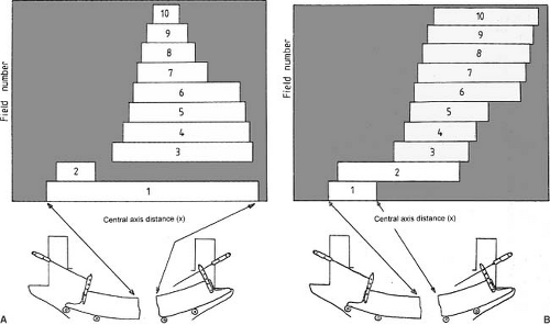Figure 20.2. Ten separate fields are stacked to generate the beam profile shown in Figure 20.1. Multileaf collimator leaves are shown schematically below the fields: A: leaf setting as “close-in” technique; B: leaf settings as “leaf-sweep” technique. (From Web S. The Physics of Conformal Radiotherapy. Bristol, UK: Institute of Physics Publishing; 1997:132, with permission.)

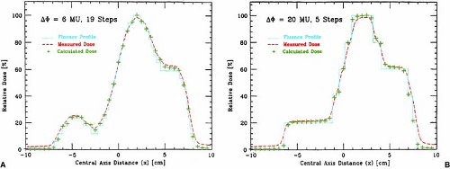Figure 20.3. Comparison of calculated fluence, measured dose, and calculated dose for the intensity-modulated profile generated by the step-and-shoot method. (From Bortfeld TR, Kahler DL, Waldron TJ, et al. X-ray field compensation with multileaf collimators. Int J Radiat Oncol Biol Phys. 1994;28:723–730, with permission.)

The leaves of a dynamic MLC are motor driven and are capable of moving with a speed of greater than 2 cm per second. The motion is under the control of a computer, which also accurately monitors the leaf positions. The problem of determining leaf velocity profiles has been solved by several investigators (12,16,17). The solution is not unique but rather consists of an optimization algorithm to accurately deliver the planned intensity-modulated profiles under the constraints of maximum possible leaf velocity and minimum possible treatment time.

The basic principle of dynamic collimation is illustrated in Figure 20.4. A pair of leaves defines an aperture with the leading leaf 2 moving with velocity V₂(x) and the trailing leaf 1 with velocity V₁(x). Assuming that the beam output is constant with no transmission through the leaves, penumbra, or scattering, the profile intensity I(x) as a function of position x is given by the cumulative beam-on times, t₁(x) and t₂(x), in terms of cumulative MUs that the inside edges of leaves 1 and 2, respectively, reach point x; that is:

Differentiating Equation 20.3 with respect to x gives:

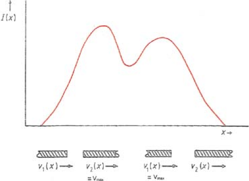Figure 20.4. Illustration of dynamic multileaf collimator motion to generate intensity-modulated profile. A pair of leaves with the leading leaf 2 moving with velocity V₂(x) and the trailing leaf 1 with velocity V₁(x). In the rising part of the fluence profile, leaf 2 moves with the maximum speed V_max, and in the falling part of the fluence, leaf 1 moves with V_max. (Adapted from Web S. The Physics of Conformal Radiotherapy. Bristol, UK: Institute of Physics Publishing; 1997:104.)

or:

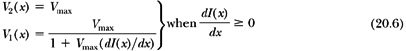
To minimize the total treatment time, the optimal solution is to move the faster of the two leaves at the maximum allowed speed, V_max, and modulate the intensity with the slower leaf. If the gradient of the profile dI(x)/dx is zero, then according to Equation 20.5, the two speeds are equal and should be set to V_max. If the gradient is positive, then the speed of leaf 2 is higher than that of leaf 1 and therefore it is set equal to V_max; and if the gradient is negative, then the speed of leaf 1 is set equal to V_max. Once the speed of the faster leaf is set to V_max, the speed of the slower leaf can be uniquely determined from Equation 20.5; that is:

and:

In summary, the dynamic MLC algorithm is based on the following principles:

If the gradient of the intensity profile is positive (increasing fluence), the leading leaf should move at the maximum speed and the trailing leaf should provide the required intensity modulation.
If the spatial gradient of the intensity profile is negative (decreasing fluence), the trailing leaf should move at the maximum speed and the leading leaf should provide the required intensity modulation.

A.3. Intensity-modulated Arc Therapy

Yu (14) has developed an intensity-modulated arc therapy (IMAT) technique that uses the MLC dynamically to shape the fields as well as rotate the gantry in the arc therapy mode. The method is similar to the step-and-shoot in that each field (positioned along the arc) is subdivided into subfields of uniform intensity, which are superimposed to produce the desired intensity modulation. However, the MLC moves dynamically to shape each subfield while the gantry is rotating and the beam is on all the time. Multiple overlapping arcs are delivered with the leaves moving to new positions at a regular angular interval, for example, 5 degrees. Each arc is programmed to deliver one subfield at each gantry angle. A new arc is started to deliver the next subfield and so on until all the planned arcs and their subfields have been delivered. The magnitude of the intensity step per arc and the number of arcs required depend on the complexity of the treatment. A typical treatment takes three to five arcs and the operational complexity is comparable to conventional arc therapy (18).

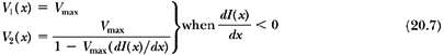
The IMAT algorithm divides the two-dimensional intensity distribution (obtained through inverse treatment planning) into multiple one-dimensional intensity profiles to be delivered by pairs of opposing leaves. The intensity profiles are then decomposed into discrete intensity levels to be delivered by subfields in a stack arrangement using multiple arcs as shown in Figure 20.5. The leaf positions for each subfield are determined based on the decomposition pattern selected. As discussed earlier, there are (N!)² possible decomposition patterns for an N-level profile (to be delivered by N arcs) of only one peak. For example, in a simple case of a one-dimensional profile with three levels (Fig. 20.5A), there are (3!)² = 36 different decomposition patterns of which only three are shown (Fig. 20.5B–D). The decomposition patterns are determined by a computer algorithm, which creates field apertures by positioning left and right edges of each leaf pair. For efficiency, each edge is used once for leaf positioning. From a large number of decomposition patterns available, the algorithm favors those in which the subfields at adjacent beam angles require the least distance of travel by the MLC leaves.

As discussed earlier, the superimposition of subfields (through multiple arcs) creates the intensity modulation of fields at each beam angle. Whereas a one-dimensional profile is generated by stacking of fields defined by one leaf pair, the two-dimensional profiles are created by repeating the whole process for all the leaf pairs of the MLC.

B. Tomotherapy

Tomotherapy is an IMRT technique in which the patient is treated slice by slice by intensity-modulated beams in a manner analogous to CT imaging. A special collimator is designed to generate the
IMBs as the gantry rotates around the longitudinal axis of the patient. In one device the couch is indexed one to two slices at a time and in the other the couch moves continuously as in a helical CT. The former was developed by the NOMOS Corporation² and the latter by the medical physics group at the University of Wisconsin.³

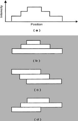Figure 20.5. Stacking of three subfields using multiple arcs. Different decomposition patterns are possible but only three are shown (b, c, d) to generate profile shown in (a). (From Yu CX. Intensity modulated arc therapy: a new method for delivering conformal radiation therapy. In: Sternick ES, ed. The Theory and Practice of Intensity Modulated Radiation Therapy. Madison, WI: Advanced Medical Publishing; 1997:107–120, with permission.)

Only gold members can continue reading. Log In or Register to continue