Introduction to IVIM MRI
Intravoxel incoherent motion magnetic resonance imaging (IVIM MRI) allows both tissue microstructure (from molecular diffusion) and tissue microcirculation (perfusion) to be investigated at once. Besides brain and head tumors perfusion-driven IVIM MRI is currently being investigated to assess malignant lesions in the liver, the prostate, or the breast or evaluate tissue function in the kidney or even the placenta or the fetus. Indeed, IVIM MRI is experiencing a remarkable revival for applications throughout the body. The first reason is certainly that vast progress has been made in MRI scanner hardware and sequence developments, satisfying the signal-to-noise-ratio-hungry IVIM method. The second reason is that diffusion MRI has become a pillar of clinical MRI, part of many protocols, so that one may get IVIM/perfusion images “for free,” together with the diffusion images, without the need for additional scanning time. Perfusion imaging, as permitted by IVIM MRI, gives valuable information on neoangiogenesis or microvascular heterogeneity, as well as on treatment efficacy of chemo- or radiotherapy, and especially the effectiveness of antiangiogenic drugs or vascular targeting agents. The third reason is that IVIM MRI does not involve contrast agents, serving as an interesting alternative to perfusion MRI in some patients with contraindications for contrast agents, such as patients with renal failure at risk for nephrogenic systemic fibrosis (NSF). Recently, an accumulation of gadolinium deposits in the brain or other organs in patients who have received multiple injections of contrast agents has been demonstrated [1, 2]. The IVIM method, thus, appears particularly appealing for patients requiring multiple MRI scans, as well as for children or pregnant patients. This section will introduce the IVIM concept. In Section II of this book other perfusion MRI methods will be presented. Section III will provide a detailed overview of the many potential clinical applications (neuro, body, and musculoskeletal) of perfusion-driven IVIM MRI that are currently under evaluation. Finally, Section IV will address methodological issues and look at further developments.
1.1 The IVIM Concept
“IVIM refers to translational movements which within a given voxel and during the measurement time present a distribution of speeds in orientation and/or amplitude” [3–5]. The concept was introduced in 1986, together with the foundation of diffusion MRI [3], as it was realized that the flowof blood incapillaries(perfusion) would mimic a diffusion process and impact diffusion MRI measurements. However, perfusion and diffusion effects can be disentangled in diffusion MRI, leading to separate maps and measurements of molecular diffusion and perfusion [4]. Diffusion and blood microcirculation are two completely different physical phenomena, taking place at very different spatial and temporal scales, but because both can be addressed with IVIM MRI, they have been associated for many years in the MRI and radiology communities where “diffusion and perfusion MRI” often appear as session titles or journal keywords.
1.1.1 Molecular Diffusion
Molecular diffusion is just one type of IVIM. Due to their thermal energy all molecules move, colliding against each other. Each collision results in a change in the motion direction of each molecule, and the overall process is well described by a random walk, as first realized by Einstein. For liquid water the average of individual molecular displacement between two “collisions,” l, in 3D space, is in the 10th of a nanometer range while mean “velocity” (a concept more valid for a gas phase than a liquid phase), v, is around 100 m/s, which correspond to a diffusion coefficient, D, around 10–9 m²/s based on Einstein equation (D = l v/6) [6]. Diffusion refers to the random movement of individual molecules, but on a statistical basis, taking into account billions of molecules, each one diffusing on its own, this movement translates into an overall probability displacement along one spatial direction that obeys a Gaussian distribution. For water at body temperature the average diffusion distance is 17 μm during a time interval of 50 ms, a perfect scale to explore the microstructure of biological tissues in vivo (Fig 1.1).
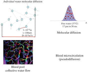
Figure 1.1 Molecular diffusion and blood pseudodiffusion. Molecular diffusion (top) is a random process at the individual molecular level. According to Einstein’s equation, the diffusion-driven distribution of molecular displacements is a Gaussian distribution of molecular displacement (free diffusion). Pseudodiffusion (bottom) for blood flow (BF) results from the collective water flow in the randomly orientated capillary segments.
1.1.2 Perfusion-Driven Pseudodiffusion
Apparent motion randomness for perfusion results from the geometry of the vessel network where blood circulates, under the hypothesis that the microvascular network can be modeled by a series of straight segments randomly oriented in space and uniformly distributed over 4π within each voxel in the 3D space Here, randomness thus results from the collective motion of blood water molecules in the network, flowing from one capillary segment to the next, in addition to the individual diffusion movement of blood water molecules This collective movement has been described as a pseudodiffusion process where the average displacement, l, would now correspond to the mean capillary segment length and the mean velocity, v, would be that of blood in the vessels (Fig 1.1) [4] Using Einstein’s diffusion equation for pseudodiffusion one gets a value for the pseudodiffusion coefficient, D* = lv/6, which is around 10–8 m²/s, taking l as 100 μm and v as 1 mm/s It is really fortunate that D* is close enough to D for it to be possible to make diffusion MRI sensitive to both diffusion and blood microcirculation, both resulting, separately, in a monoexponential decay of the MRI signal with the b value (see below) But the blood microcirculation component decays 10 times faster, which allows the two independent phenomena to be separated Interestingly, the value for D* is found to be similar across other species that have been scanned, which is not completely surprising as small animals have shorter capillary segments but higher flow velocities [7].
1.1.3 Other Sources of IVIM
By definition IVIM does not specifically refer to diffusion and blood microcirculation, and other sources of IVIM are possible. Some examples are given at the end of this chapter, especially in the domain of virtual elastography, but the chapters of this book will exclusively focus on perfusion-driven IVIM.
1.2 IVIM MRI
1.2.1 IVIM Contribution to the MRI Signal
The random displacement of individual molecules results in a signal attenuation in the presence of magnetic-field-encoding gradient pulses. This attenuation increases with the diffusion coefficient and the degree of sensitization to diffusion of the MRI pulse sequence (so-called b value, which depends on the gradient pulse shapes, duration, and separation times; see Refs. [3, 4]). With free (Gaussian) molecular diffusion the overall MRI signal attenuation, S(b)/S(0), follows a monoexponential decay [3]:
(1.1)
where S(b) and S(0) are the MRI signal intensities at a given b value and b = 0, respectively. In the presence of blood microcirculation, the overall MRI signal attenuation, S(b)/S(0), becomes the sum of two exponentials (biexponential decay), one for tissue diffusion and one for the blood compartment (assuming water exchange between blood and tissues is negligible during the encoding time, a hypothesis which has not yet been deeply investigated):
(1.2)
where f IVIM is the flowing blood fraction (sometimes also called f p, or even simply f), D* is the pseudodiffusion coefficient ascribed to blood random microcirculation, D is the water diffusion coefficient in the tissue, and D b is the water diffusion coefficient in blood (as diffusion of individual water molecules also occurs in blood). Because the fraction of the flowing blood is usually small (a few percent) compared to the overall tissue water content, the perfusion-driven IVIM signature appears more as a deviation as small b values of the tissue diffusion–driven monoexponential signal decay (Fig 1.2).
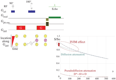
Figure 1.2 Effects of diffusion and pseudodiffusion on the MRI signal. Random water displacements (either from individual molecular motion or from collective water incoherent flow at the voxel level) result in an exponential decay of the signal amplitude with the degree of field gradient encoding (b value). The tissue diffusion and BF component contribute separately to the signal, resulting in a biexponential shape. However, as D*>>D the IVIM (BF) effect appears as a deviation of the tissue diffusion signal decay at low b values.
1.2.2 Extracting Diffusion and Perfusion Parameters
When both diffusion and flowing blood effects are present the apparent diffusion coefficient, ADC [3], calculated from signals S(b) and S(0) as ln[S(b)/S(0)]/b is higher than D. This difference is mostly seen when using small b values. As f IVIM is usually small, one has ADC ≈ D + f IVIM/b, and f IVIM simply appears as the (negative) intercept of the diffusion component of the signal decay in log plots with b values (Fig 1.3) [4].
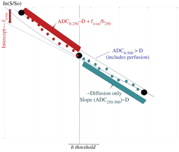
Figure 1.3 Strategies to process IVIM/diffusion data sets. Above a given threshold (which depends on the tissue IVIM/diffusion intrinsic parameters) for the b values only tissue diffusion contributes to the signal decay. The ADC obtained with b values higher than this threshold (e.g., ADC250–500) is the tissue diffusion coefficient, D. At lower b values (e.g., ADC0–250) the ADC includes the BF component. Hence, the flowing blood fraction (f IVIM, which is the intercept of the tissue diffusion decay curve) can be obtained from those two ADC values, making only three b values in total. Alternately, one may prefer fitting the overall signal attenuation curve with an IVIM/diffusion model. To reduce the effect of noise, one often performs fitting in two steps, first estimating diffusion from high b value signals, then subtracting the tissue diffusion component from the overall signal to estimate the IVIM parameters.
On the basis of this observation, the first perfusion-driven IVIM measurements were obtained just by using three b values (0, 100, and 200 s/mm², the highest achievable value with the hardware available at that time) [4] (Fig 1.3). The three b values scheme used at the beginning of IVIM MRI has gained popularity recently although with the larger gradient strengths available, as this approach minimizes acquisition times. The IVIM concept was first validated in a dedicated phantom (Fig. 6 in Ref. [4]) and in a small series of patients with tumors [4]. Phantoms mimicking both perfusion and tissue diffusion are tricky to make. We used calibrated sephadex beads, inside which water could diffuse and between which a flow of water was maintained, mimicking random flow in capillaries. The IVIM concept was further confirmed by other groups in normal subjects and animal models [8–11].
IVIM really entered the clinical world when echo-planar imaging (EPI) became available, as a signal acquired at multiple and higher b values could be obtained free of motion artifacts [12], allowing the first clinical validation of IVIM perfusion MRI in a series of patients with liver lesions [13]. If one considers that IVIM effects are completely negligible for b values above 250 mm²/s (see below) the slope of the signal attenuation between b = 250 and, say, 500 s/mm² is, according to Eq. 1.2, just the tissue diffusion coefficient D: ADC250–500 ≈ D, while ADC0–250 ≈D + f IVIM/250. The perfusion fraction would then come as 250 ×(ADC0–250 – ADC250–500), where the ADC is defined as:
(1.3)
However, D* cannot be estimated with this simplistic approach. Furthermore, parameter estimates could be noisy unless one acquires multiple signals at those three b values and average them out. Then, the total acquisition time increases, and considering three repeated acquisitions for each of the 3b values, becomes identical to the acquisition of signals at 15 different b values. With so many acquired signals at hand one may rather consider fitting those signals with the IVIM/diffusion model. Equation 1.2 can be rewritten more generally as:
(1.4)
Here S 0diff and S 0IVIM are the fractions of pure diffusion and IVIM components to the overall signal, respectively, with S 0diff = S(0)(1 – f IVIM) and S 0IVIM = S(0)f IVIM. F diff(b) and F IVIM(b) are, respectively, the diffusion and perfusion-related IVIM signal attenuation as a function of diffusion weighting (b value). It should be noted here that tissue and blood contribute to S(0) with different T2 and T1 weightings, which means that f IVIM values might be misestimated, depending on the echo time (TE), and the field strength Bo, as well as the tissue voxel content (e.g., local blood oxygen level), an issue when comparing literature results (see also Chapter 19 about this issue). With the pseudodiffusion model introduced above, the expression for F IVIM(b) is simply:
(1.5)
However, other models can be used, such as the “sinc” model introduced later in this chapter or in more detail in Chapter 19.
As for the diffusion component, with the common monoexponential model one has, as in Eq. 1.1:
(1.6)
where D is the diffusion coefficient of water in the tissue. Here also, other models are now being used, especially when using high b values, as the monoexponential model assumes diffusion is Gaussian (free), which is far from the case in biological tissues and an important source of errors in the estimation of IVIM parameters (see below).
With a dataset comprising signals acquired at multiple b values one may get estimates of S(0), f IVIM, D*—usually D b is included in D* but might be estimated [14]—and D by fitting the signal with Eq. 1.2 or 1.4. However, the fitting process is known to be sensitive to noise (and then to local minima) and may lead to erroneous or inaccurate parameter estimates if the number of acquired signals is not very large compared to the number of parameters to estimate. Considering that the IVIM component become negligible at some point when b increases (as D* is much higher than D), a popular, elegant, and more robust approach is to split the signal in two parts and switch to a two-step fitting process, first fitting the experimental data for high b values (above 200–600 s/mm²) with the diffusion model for F diff(b) and then fitting the residual signal after removing the diffusion component at low b values [15] with the IVIM model F IVIM(b).
For this two-step approach, one needs to determine the threshold b value that separates the pure diffusion part and the IVIM/diffusion mixed part. Unfortunately, there is no generic response, as this threshold value depends highly on the parameters one has to estimate, f IVIM, D*, and D. In the normal brain f IVIM is less than 5% and D is around 0.001 mm²/s, so the IVIM component accounts for less than 0.3% of the signal for b > 200 s/mm². In body tissues, however, f IVIM values as high as 20% are not uncommon while D may be on the order of 0.002 mm²/s, so the IVIM component at b = 400 s/mm² may still be around a few percent and higher threshold b values might be required. Hence, the b value threshold should be chosen according to the expected level of perfusion (low in the brain, higher in the body) and, of course, the overall signal-to-noise ratio (SNR) of the data.
In summary, there is no consensus, yet, on the best processing approach of IVIM data. There is extensive literature investigating the pros and cons of fitting algorithms, simultaneous or multistep [16, 17], as well as other methods, such as the Bayesian algorithm [18–21] or even an adaptive thresholding approach [20]. Those approaches will be reviewed in detail in Section IV of this book.
1.3 Pitfalls to Consider for an Accurate Estimation of Perfusion-Driven IVIM Parameters
1.3.1 Non-Gaussian Tissue Diffusion
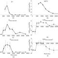
An accurate estimation of the IVIM parameters first requires proper handling of the diffusion component within the IVIM/diffusion MRI signals that account generally for more than 90% of the total signal at low b values. Although the ADC concept has been (and still is) extremely useful, it does not provide a precise estimate of the diffusion-sensitive MRI signal decay. Because the diffusion process in tissues is not Gaussian and the semi log plot of the signal decay, F diff, in biological tissues is not straight (as assumed intrinsically by the ADC and Eq. 1.6) but exhibits a curvature [22] (Fig 1.4). In the presence of non-Gaussian diffusion, the use of Eq. 1.6 to fit the diffusion component of the signal above the b value threshold will introduce a significant bias to the estimated perfusion parameters: Fitting the curved diffusion signal attenuation with a straight line (in log plots) according to Eq. 1.6 results in an artifactual IVIM effect, as acquired data points at low b values will automatically appear above the fitted diffusion signal decay (Fig 1.4). The perfusion fraction, f IVIM, will, thus, be overestimated. Furthermore, the shape of the residual signal decay at low b values will appear close to an exponential, mimicking Eq. 1.5, which would be misleading (D* values would be overestimated as well).
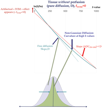
Figure 1.4 Non-Gaussian diffusion. Failing to take into account non-Gaussian diffusion effects might lead to erroneous f IVIM and D* parameter estimates (overestimation), as shown here in a simulated tissue model without perfusion. Non-Gaussian diffusion that becomes visible at high b values originates from the interaction of water-diffusing molecules with obstacles, such as cell membranes, and results in a curvature of the signal attenuation. Modeling the tissue diffusion component with a monoexponential model underestimates genuine diffusion (ADC < D) when the signal at high b values is included, which, in turn, creates an artifactual IVIM effect (left). Non-Gaussian diffusion must be properly handled using adequate models, such as the kurtosis model or other models, to avoid such erroneous IVIM effects.
Related posts:
 IVIM MRI: A Window to the Pathophysiology Underlying Cerebral Small Vessel Disease
 Clinical Applications of IVIM MRI to the Nervous System
 Head and Neck IVIM MRI
 Perfusion Marries Diffusion: Arterial Spin Labeling Prepared IVIM
 IVIM MRI in the Kidney
 Clinical Application of IVIM in the Female Pelvis
Stay updated, free articles. Join our Telegram channel

Full access? Get Clinical Tree


