IVIM Models: Advantages, Disadvantages, and Analysis Pitfalls

Gabrielle Fournet, Luisa Ciobanu, and Denis Le Bihan

NeuroSpin/Joliot/CEA Saclay, Bat 145, 91191 Gif-sur-Yvette, France

Since its introduction by Le Bihan et al. in 1988 [1], the perfusion- driven monoexponential intravoxel incoherent motion (IVIM) model has been widely used, especially for medical applications. However, over the years, other models have emerged. This chapter aims to describe the evolution of IVIM models and present their respective advantages and disadvantages. The quality of the analysis method used together with the IVIM model is also essential. The second part of this chapter gives a review of the possible analysis methods, and, finally, the third part covers some of the analysis pitfalls.

19.1 IVIM Models

For notation purposes, the diffusion component will be labeled F _Diff and the IVIM component F _IVIM so that the total signal acquired with a diffusion-weighted (DW) sequence, S, can be expressed as

(19.1)

S ( b ) = ( 1 – f IVIM ) · F Diff ( b ) + f IVIM · F IVIM ( b ) ,

where b is the diffusion weighting, also called the b value, and f _IVIM the flowing blood volume fraction.

In this section, we will focus on IVIM models. First, we will present the two models originally introduced by Le Bihan et al. [1] Then, considerations leading to the emergence of other types of models, intermediate and multicompartment models, are presented. Finally, we show how the T ₁/T ₂ dependence of the blood and tissue compartments can be incorporated into the IVIM model.

19.1.1 The Two Original Models

Making the hypothesis that the microvascular network can be modeled by a series of straight segments randomly oriented in space and uniformly distributed over 4π within each voxel in the 3D space, the expression for the IVIM signal as a function of diffusion weighting F _IVIM(b) depends on the mean vessel segment length l, the mean blood flow velocity V, and the diffusion encoding time. Two limit cases can be defined.

19.1.1.1 The exponential model

The original IVIM model assumes that blood flow changes directions several times during the diffusion time, as shown in Fig 19.1a. In this case, the isochromat trajectories can be modeled as random walks, thereby adding up to a process that resembles diffusion and is commonly called “pseudodiffusion.” In this case, F _IVIM(b) can be expressed as

(19.2)

F IVIM ( b ) = e – b ( D b + D ∗ ) ,

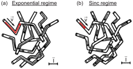
Figure 19.1 Representation of isochromats flowing in a capillary network. Each arrow corresponds to one isochromat trajectory in the capillary network during the diffusion encoding time. In the case of the exponential regime (a), the arrows and thus trajectories consist of two or more segments. The isochromats see several vessel segments during the diffusion time. On the contrary, in the sinc regime (b), the arrows always appear in a single segment; therefore, isochromats stay in the same capillary segment during the diffusion encoding time. The scale bar represents the mean capillary segment length. Adapted from Ref. [1].

where D _b is the diffusion coefficient of water in blood and D* the pseudodiffusion coefficient.

The expression for D* can be found by going back to Einstein’s equation [2]

(19.3)

D ∗ = lV 6 ,

where l is the mean vessel segment length instead of the mean intermolecular distance and V the mean blood velocity (in three dimensions).

This model represents one of the two limit cases, namely, it is valid when the measurement time (“diffusion time”) is long, the blood flow velocity is fast, or the vessel segments are short.

19.1.1.2 The sinc model

The second model is valid when blood never changes vessel segments during the measurement time, that is, when segments are long, the blood flow velocity is slow or the diffusion time is short, as shown in Fig 19.1b.

The phase shift Φ of the transverse magnetization due to spin motion between t = 0 and t = TE (echo time) for a spin-echo sequence can be expressed as

(19.4)

Φ = γ ∫ 0 TE 2 – V → · G → · t · d t + ∫ TE 2 TE V → · G → · t · d t ,

where γ is the proton gyromagnetic ratio, V → the instantaneous velocity vector, and G → the instantaneous magnetic field gradient.

Introducing the angle between the direction of a capillary segment and the gradient direction θ, Eq. 19.4 can be simplified to

(19.5)

Φ = c · V · cos ( θ ) ,

with

(19.6)

c = γ ∫ 0 TE 2 – G · t · d t + ∫ TE 2 TE G · t · d t .

To obtain the expression for F _IVIM, Eq. 19.5 needs to be generalized for a distribution of capillary orientations ρ(θ, ξ) in the voxel in 3D and a velocity distribution p(V):

(19.7)

F IVIM = ∫ 0 ∞ ∫ 0 2 π ∫ 0 π e i · c · V · cos ( θ ) · p ( θ , ξ ) p ( V ) sin ( θ ) d θ d ξ d V .

In this regime and if the blood flow velocity is assumed to be constant, F _IVIM becomes a sinc function

(19.8)

F IVIM ( c ) = e – b D b · sin c( c V ) .

A pseudodiffusion coefficient D*_sinc can also be defined in this regime by calculating the Taylor expansion limited to the first orders of F _IVIM(c) (neglecting D _b)

(19.9)

F IVIM ( c ) = 1 – ( c v ) 2 3 ! + o ( c v ) 4 ,

and comparing it to the Taylor expansion limited to the first orders of F _IVIM in Eq. 19.2 (neglecting D _b),

(19.10)

F IVIM ( b ) = 1 – b D ∗ + o ( b D ∗ ) 2 .

This gives

(19.11)

D sinc ∗ ∼ c 2 v 2 6 b .

For a basic pulsed-gradient spin-echo (PGSE) sequence (with δ and Δ= gradient pulse duration and separation interval, respectively),

(19.12)

c = γ G δ Δ . .

In the short pulse approximation, δ << Δ, b ≅ γ ² G ² δ ²Δ, and D*_sinc simplifies to

(19.13)

D sinc ∗ ∼ v 2 D 6 .

It can be noticed that D sinc ∗ is independent of l as spins never get to probe the entire capillary segment.

As often, the real situation probably lies between these two extreme models. The transition between the sinc and exponential regimes can be studied both analytically and numerically, and several approaches have been proposed to handle this intermediate case (see Section 19.1.2). Without considering the exponential term for the dependence of F _IVIM(c) on D _b and using the short pulse approximation (Δ+δ~Δ), the magnetic resonance imaging (MRI) signal corresponding to an isochromat that sees an N number of segments during the diffusion encoding time Δ, S _IC(b), can be expressed as a product of sinc functions:

(19.14)

S IC ( b ) = sinc v b Δ N N .

As N goes to infinity, the equation for S _IC(b) becomes exponential and the expression for D* in the exponential regime can be recovered:

(19.15)

lim N → ∞ S IC ( b ) = e b v 2 Δ 6 N = e – bvl 6 .

Using numerical simulations of a random walk of molecules in a network of a varying number N of randomly oriented capillary segments, Fig 19.2 illustrates the transition from the sinc to the exponential regime. The signal attenuation becomes monoexponential for N ≥ 5 capillaries for the example shown.

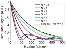
Figure 19.2 Evolution of the simulated signal versus b value with N = V(∆+δ)/l, the number of segments seen by an isochromat during ∆+δ. N is varied by changing the segment length l and keeping the blood flow velocity V at 3 mm/s, δ = 3 ms, and ∆ = 14 ms. For N = 5, exp(–bD*) with D* = lV/6 has been added to show that the simulated signal becomes exponential for this N value (difference between the two curves <3%).

Performing numerical simulations of a random walk of molecules in a network of randomly oriented capillary segments [3], it is possible to show that, when considering a Gaussian distribution of blood flow velocities instead of a constant blood flow velocity, the IVIM signal plotted against the b value looks “exponential” even though isochromats do not change direction many times (sinc regime). Figure 19.3 displays this phenomenon, which is coherent with results from the literature [4, 5].

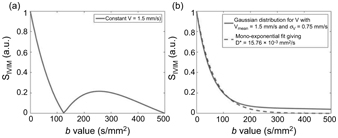
Figure 19.3 Plot of the IVIM signal in the sinc regime for d = 3 ms, D = 34 ms, and (a) a constant V = 1.5 mm/s or (b) a Gaussian distribution for V with V _mean = 1.5 mm/s, s _V = 0.5· V _mean, and 1000 samples of V. In (b), a monoexpo- nential fit of the IVIM signal was added. It gives D* = 15.76·10⁻³ mm²/s.

Therefore, in practice, if there is a Gaussian distribution of the blood flow velocity in the vessel network, it is not possible to distinguish between a sinc and an exponential curve. This likely explains why the sinc model has never been observed experimentally.

But then, in the intermediate regime, the IVIM signal would be in between the true pseudodiffusion model (D* only depends on the capillary geometry and flow) and the distributed sinc model (D* also depends on the acquisition parameters, mainly the measurement time). Hence, other intermediate regime models have been proposed.

19.1.2 Intermediate Models

Kennan et al. [6] have presented a model based on a velocity autocorrelation function to cover intermediate situations between the two extreme regimes, exponential and sinc.

Kennan’s model uses a velocity autocorrelation function to describe the isochromats’ dynamics. The velocity autocorrelation function is a measure of velocity fluctuations in the capillary network and is defined as the average of the scalar product of the v_{_}eloci_.ty of_{_.}an isochromat evaluated at different times t and t ^’: ⟨ V ( t ′ ′ ) ¯ · V ( t ′ ) ¯ ⟩ . . For a capillary network with a distribution of segments with different lengths, this product can be expressed as

(19.16)

⟨ V ( t ′ ′ ) ¯ · V ( t ′ ) ¯ ⟩ = ⟨ V ¯ ⟩ e t – t ′ T 0 ,

where ^· ⟨ V ¯ 2 ⟩ is the mean squared blood flow velocity and T ₀ the correlation time that corresponds to the average time the isochromats stay in a given segment.

After integrating the expression of the signal attenuation for a PGSE sequence and the assumed velocity autocorrelation function in Eq. 19.16, the IVIM signal becomes

(19.17)

F IVIM ( b ) = e – b ⟨ V ¯ 2 ⟩ 3 T 0 Ω + D b ,

where Ω is a function of δ, Δ, and T ₀.

The parameters extracted from this model are ⟨ V ¯ 2 ⟩ , T ₀, and the mean segment length l, which can be estimated by the relation

(19.18)

l = 2 T 0 V ¯ 2 ,

This model converges toward the exponential and the sinc regimes at long and very short diffusion times, respectively, and is expected to also cover intermediate regimes. When comparing the standard monoexponential IVIM model to Kennan’s model, the models are very similar except that D* has been replaced by ⟨ V ¯ 2 ⟩ T ₀ Ω/3.

The validity of the Gaussian phase approximation used by Kennan et al. has been questioned by Wetscherek et al., who suggested a different model (see Chapter 21). Arguing that the assumption that isochromats change direction enough times during the diffusion encoding time to mimic a diffusion process is invalid in some cases, Wetscherek et al. introduced a model to describe the signal attenuation of the perfusion fraction in-between the two original models based on normalized phase distributions [5]:

(19.19)

F IVIM ( b ) = F ( b , V , T , τ ) e – b D b ,

where

(19.20)

F ( b , V , T , τ ) = ∫ – ∞ + ∞ p φ , T τ e i V bT φ d φ ,

with τ = l/V, T the total duration of the diffusion gradients, φ the normalized phase, and ρ(φ,T/τ) the phase distributions.

To obtain F(b,V,T,τ), only the phase distribution for the applied diffusion gradient profile and the number of directional changes N = T/τ need to be calculated. Since at short and long diffusion encoding times, the sinc and exponential models can be recovered from the proposed model, it is also assumed to describe well the intermediate regime. Wetscherek et al. proposed to estimate τ and V directly, instead of their combination through D* = τV ²/6, to obtain a more detailed description of the incoherent motion by combining flow-compensated and non-flow-compensated diffusion gradients, but this method is out of the scope of this chapter and will be discussed in Chapter 21.

The models described so far assume a single IVIM compartment. However, in biological tissues, the existence of multiple compart- ments must be considered.

19.1.3 Multicompartment Models

Using innovative ways to isolate the signal coming from flowing blood from that coming from static tissue, a number of authors have shown that there might be several vascular compartments to consider instead of just one when describing the IVIM signal.

Neil et al. developed a strategy to directly suppress the diffusion component by injecting a contrast agent intravenously [7]. The IVIM signal they obtained was better fitted to a biexponential model. Their hypothesis for this second exponential in the IVIM signal is that it is associated with an incompletely suppressed signal from nonflowing blood. In a second experiment, the contrast agent was replaced by perfluorocarbon (PFC) to test this hypothesis [8]. Once again, a biexponential model was found to better describe the IVIM signal, invalidating the previous hypothesis and instead suggesting that multiple vascular pools could be observed within the IVIM signal.

On the basis of Neil’s findings, Henkelman et al. have suggested an IVIM model that takes into account not only capillaries but all types of vessels, including larger vessels [10]. However, the blood flow estimated with their model is one order of magnitude lower than the one reported in the literature (12 mL/min/100 g compared to 130 ± 50 mL/min/100 g), suggesting that large vessels likely do not contribute to the IVIM effect.

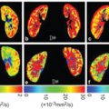
Duong et al. took inspiration from Neil’s PFC experiments and exploited the fact that the spin-lattice relaxation rate of the PFC correlates linearly with the dissolved oxygen concentration [11]. This allowed them to link each of the pseudodiffusion coefficients of the biexponential IVIM model to the arterial and venous trees and measure the associated regional arterial and venous blood volume fractions.

Recently, we established that the perfusion-driven IVIM signal could, indeed, be better described by a biexponential model at short diffusion times. This model assumes the coexistence of a slow and a fast flow pool [3]

(19.21)