10 Kidneys
 Organ Boundaries
LEARNING GOALS
 Locate and identify both kidneys.
 Demonstrate both kidneys in their entirety.
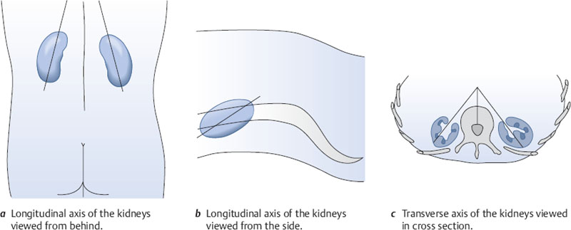
The kidneys are located in the retroperitoneum, one on each side of the spinal column. Ribs extend forward and downward over the kidneys, covering the upper third of each organ. The longitudinal axes of the kidneys converge toward the spinal column at an acute angle when viewed from behind and from the side (Fig. 10.1a,b). Their transverse axes form an approximately 45° angle with the sagittal plane (Fig. 10.1c).
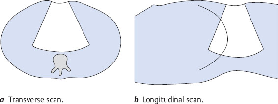
The liver, gallbladder, and pancreas are scanned primarily in transverse and longitudinal planes through the upper abdomen (Fig. 10.2).
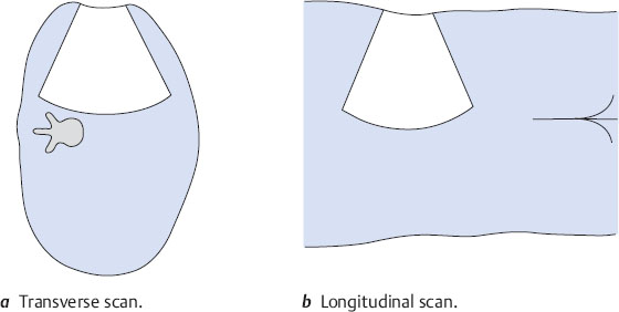
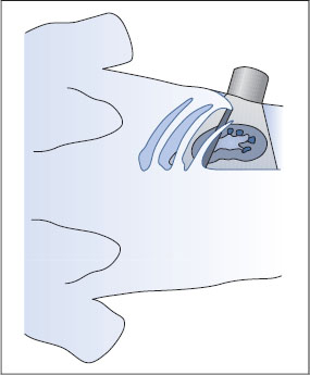
Renal scanning differs from this in several details because the kidneys are scanned from the flank. In the case of the right kidney, this means that a transverse scan is oriented as if the viewer were looking up into the sectioned torso from below (Fig. 10.3a). A longitudinal scan is like looking from posterior to anterior (Fig. 10.3b).
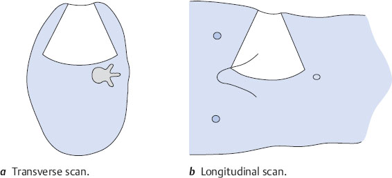
In the case of the left kidney, a transverse scan is like looking up into the torso from below (Fig. 10.4a), as on the right side. But a longitudinal scan from the left side is like looking from anterior to posterior (Fig. 10.4b).
Locating the right kidney
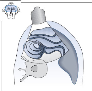
The right kidney lies posteriorly in an angle between the spinal column, musculature, and right lobe of the liver (Fig. 10.5). The right hepatic lobe extends laterally to the lower third of the kidney. The kidney is covered anteriorly by the right lobe, and its lower half in particular is covered by the right colic flexure and duodenum. Generally, then, the best approach is to scan the right kidney through the intercostal spaces from the posterolateral side and to use the liver as an acoustic window. Occasionally, however, you can obtain a clear view of the right kidney by scanning from the anterior side in thin, non-bloated patients.
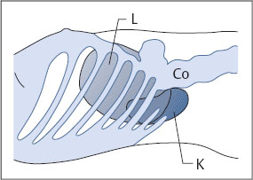
Fig. 10.5 Lateral approach to the right kidney (K). The ribs and colon (Co) obstruct vision, while the liver (L) provides an acoustic window.
Barriers to scanning
Visualization of the right kidney is obstructed by the 11th and 12th ribs and bowel gas.
Optimizing the scanning conditions
In most cases it is very helpful to have the subject take a deep breath. The kidney will move as much as several centimeters with respiratory excursions. Also, the left lateral decubitus position is preferred for renal scanning and may be supported by placing a roll beneath the contralateral side (“scoliosis” position). The ipsilateral arm can be raised to widen the intercostal spaces.
Organ identification
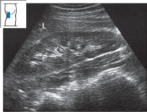
Place the transducer approximately on the posterior axillary line. Improve scanning conditions by using the maneuvers described above. Angle the scan slightly toward the head (Fig. 10.6). Define the kidney in an approximate longitudinal scan. Keep in mind that the image on the screen represents a posterior-to-anterior view of the body. Figure 10.7 illustrates the typical appearance of this scan.
You should understand that this scan does not provide either an exact longitudinal or transverse view of the kidney, as it is slightly oblique. For the time being, however, it is entirely adequate for identifying the organ.
Imaging the entire right kidney
Longitudinal flank scan of the right kidney
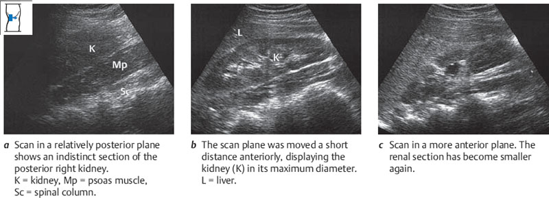
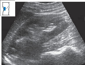
Once you have defined the right kidney in an approximately longitudinal scan on the midaxillary line as described above, scan slowly across the organ from its posterior to anterior border, repeating this pass several times (Figs. 10.8, 10.9). Notice how the renal section becomes larger and then smaller as you scan through the organ. Notice, too, whether the scan covers the entire kidney; if it does not, examine the upper pole first and then scan the lower pole. Overlying ribs are not a serious problem, as you can examine the hidden portions of the kidney in a second pass.
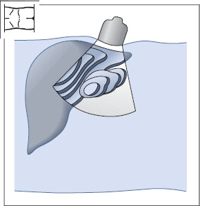
Fig. 10.8 Longitudinal flank scan: the beam is swept across the right kidney from posterior to anterior.
Transverse flank scan of the right kidney
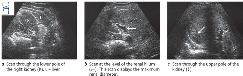
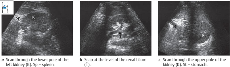
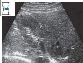
Now rotate the transducer under vision to a transverse scan of the kidney (Fig. 10.10). Notice that the left side of the image is posterior and the right side is anterior. Place the transducer just below the costal arch or in a distal intercostal space. Sweep through the kidney from lower pole to upper pole, repeating this pass several times (Fig. 10.11). As you scan through the organ, make sure that you see a complete section of the kidney on the screen. Notice that the lower renal sections are closer to the transducer (i.e., the top of the image) than the higher renal sections because the long axis of the kidney is angled toward the spine.
Locating the left kidney
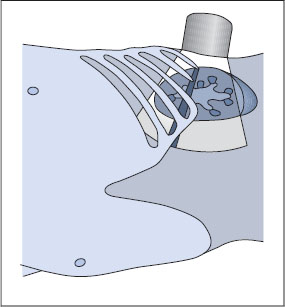
The left kidney lies posteriorly in an angle between the spinal column, musculature, and spleen (Fig. 10.12). The spleen extends laterally to about the middle of the left kidney. The lower half of the kidney is covered by the descending colon and left flexure. The left flexure passes around the anterior surface of the kidney and is in contact with it. The stomach overlies the front of the upper pole. Like the right kidney, then, the left kidney is best scanned through a posterolateral approach using the intercostal spaces and spleen as acoustic windows. The left kidney is considerably more difficult to scan than the right kidney, however, mainly because of intervening gas.
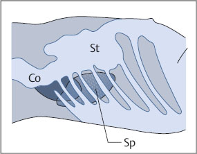
Fig. 10.12 Lateral approach to the left kidney. Colon (Co), stomach (St), and ribs obscure the left kidney, while the spleen (Sp) provides an acoustic window for scanning the upper pole.
Barriers to scanning
The main barriers to scanning the left kidney are the 11th and 12th ribs and gas in the stomach and bowel.
Optimizing the scanning conditions
The measures are the same as for the right kidney.
Organ identification
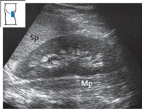
The technique for identifying the left kidney is analogous to that used on the right side. The protocol is basically the same (Fig. 10.13). Please note that a longitudinal flank scan on the left side displays the body section as if it were viewed from the front. This is opposite to the back-to-front perspective that you saw in the right renal scan. Figure 10.14 illustrates the typical appearance of the scan.
Imaging the entire left kidney
This technique is fully analogous to that used for imaging the right kidney.
Longitudinal flank scan of the left kidney
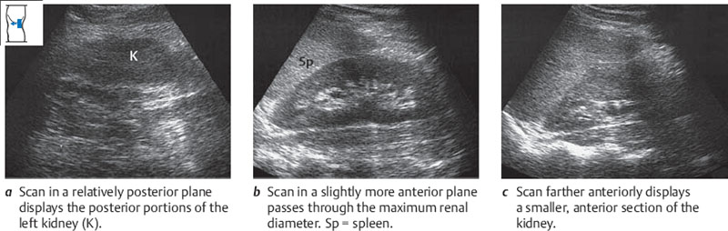
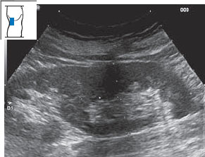
Figures 10.15 and 10.16 show how the kidney is scanned longitudinally from the flank. You scan completely through the kidney from back to front, repeating the pass several times.
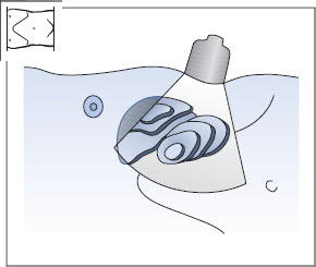
Fig. 10.15 Longitudinal flank scan: the beam is swept across the left kidney from posterior to anterior.
Transverse flank scan of the left kidney
The technique for scanning the left kidney in transverse sections is analogous to that used on the right side (Figs. 10.17, 10.18), but there is one essential difference; the left side of the screen image is anterior and the right side is posterior.
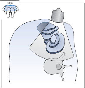
Fig. 10.17 Transverse flank scan: the beam is swept through the left kidney from lower to upper pole.
Abnormalities in locating the kidneys
Renal agenesis and ectopic kidneys. In renal agenesis, one kidney is absent while the contralateral kidney is usually enlarged. Ectopic kidneys may be found in the pelvis, but often they are obscured by intervening bowel gas.
 Organ Details
KEY POINTS
Renal dimensions have the following normal ranges:
Length 9–11 cm
Width 4–7 cm
Thickness 3–5mm
LEARNING GOALS
 Evaluate the shape and size of the kidneys.
 Evaluate the renal parenchyma.
 Evaluate the renal sinus.
Size and shape of the kidneys
The kidney is a bean-shaped organ with a smooth surface that may have small indentations.
Determining renal size with ultrasound
The kidney can be measured in three dimensions: length, width, and thickness. The longitudinal flank scan is best for determining renal length (Fig. 10.19), while the transverse flank scan is best for measuring width and thickness (Fig. 10.20). For convenience, however, both length and width are often measured in the longitudinal scan.
Changes in shape and size
Changes in shape. It is not uncommon to find surface indentations in the kidney, especially in older patients (Fig. 10.21). Pyelonephritis can also lead to surface indentations. The parenchyma of the left kidney often forms a bulge opposite the border of the spleen, creating a “dromedary hump” (Figs. 10.22, 10.23).
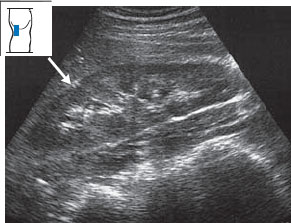
Fig. 10.21 Normal finding. A small, echogenic indentation (↓) is seen between the upper and middle groups of calyces.
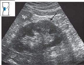
Fig. 10.22 Dromedary hump. A bulge in the renal border (↓), isoechoic to the rest of the parenchyma, appears below the border of the spleen (Sp).
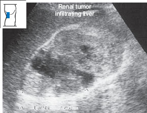
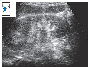
In horseshoe kidney, the two kidneys are fused at their lower poles by an isthmus of parenchyma. This creates a “horseshoe” appearance when viewed from the front. The isthmus runs anterior to the aorta and may present as a mass when the aorta is scanned (see p. 42, Fig. 10.24). Hypernephroma can also produce a bulging renal contour (Figs. 10.25, 10.27). The differential diagnosis should include a parenchymal lobule, which is easily mistaken for a tumor (Fig. 10.26). Table 10.1 lists the sonographic features of hypernephroma.
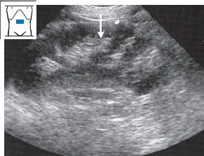
Fig. 10.24 Horseshoe kidney. The kidneys are fused by an isthmus of parenchyma (↓) that runs anterior to the aorta.
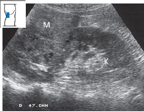
Fig. 10.25 Hypernephroma. The tumor appears as an approximately isoechoic, inhomogeneous mass on the upper pole of the right kidney. M = mass, K = kidney.
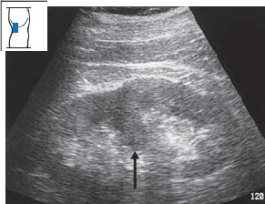
Fig. 10.26 Parenchymal lobule. Despite its resemblance to a tumor in this plane of section, the mass protruding into the renal pelvis is actually a lobule of renal parenchyma (↑).
| Hyperechoic and/or hypoechoic |
| Nonhomogeneous |
| Bulge in renal outline |
| Scalloped |
Small kidney. The kidneys may become small or shrunken (Figs. 10.28, 10.29) as a result of chronic renal disease: glomerulonephritis, pyelonephritis, or renal artery stenosis. A small kidney can also result from ageing (Fig. 10.30) and occasionally occurs as a normal variant, in which case the contralateral kidney is usually hyperplastic.
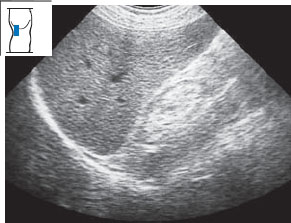
Fig. 10.28 Shrunken kidney. Ultrasound shows a markedly small kidney with lack of corticomedullary differentiation.
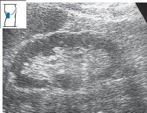
Fig. 10.29 Small kidney in a patient with a long history of insulin-dependent diabetes mellitus. Note the thinned parenchyma and loss of corticomedullary differentiation.
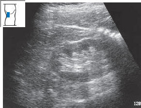
Fig. 10.30 Age-related changes. Thinning of the renal parenchyma is common with ageing, as in this 90-year-old woman.
Enlargement. Bilateral renal enlargement is seen in acute nephritis (Fig. 10.31) and renal shock as well as in chronic diseases such as diabetic nephropathy.
Renal parenchyma and renal sinus
When you slice the kidney in half in the coronal plane, you first recognize the parenchyma and the renal sinus (Fig. 10.32a). The parenchyma consists of the cortex and medulla. The medulla is composed of 8 to 20 medullary pyramids (Fig. 10.32b). The cortex is 5–7mm thick and forms the outer layer of the renal parenchyma. Fingers of cortex called the renal columns extend between the pyramids (Fig. 10.32c). The renal sinus contains the renal pelvis, a flattened sac into which the calyces open (Fig. 10.32d). The renal pelvis is surrounded by fat, connective tissue, and vessels (Fig. 10.32e, f).
Related posts:
Stay updated, free articles. Join our Telegram channel

Full access? Get Clinical Tree


