1. Magnetism A fundamental property of matter generated by moving charges, usually electrons. Magnetic properties of materials result from the organization and motion of the electron.
2. Magnetic fields
a. Magnetic fields exist as dipoles and can be induced by a moving electric charge in a wire (Fig. 12-1).
b. Units of magnetic fields are tesla (T) and gauss (G): 1 T = 10,000 G.
c. The earth’s magnetic field is 0.5 G or 5 mT; A 1.5 T MRI scanner has 30,000 times stronger field.
3. Magnetic properties of materials Magnetic susceptibility describes the extent to which a material becomes magnetized in a magnetic field.
a. Diamagnetic materials have negative susceptibility and oppose the magnetic field (Fig. 12-2, left).
(i) Examples of diamagnetic materials are calcium, water, and most organic materials.
b. Paramagnetic materials have positive susceptibility and enhance the magnetic field (Fig. 12-2, right).
(i) That is, molecular oxygen (O2), deoxyhemoglobin, methemoglobin, and gadolinium-based agents
c. Ferromagnetic materials are “superparamagnetic” and augment the magnetic field substantially.
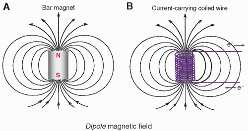
▪ FIGURE 12-1 A. The magnetic field has two poles with magnetic field lines emerging from the north pole (N) and returning to the south pole (S), as illustrated by a simple bar magnet. B. A coiled wire carrying an electric current produces a magnetic field with characteristics similar to a bar magnet. Magnetic field strength and field density are dependent on the amplitude of the current and the number of coil turns.

▪ FIGURE 12-2 The local magnetic field can be changed in the presence of diamagnetic (depletion) and paramagnetic (augmentation) materials, with an impact on the signals generated from nearby signal sources such as the hydrogen atoms in water molecules.
4. Magnetic characteristics of the nucleus
a. The nucleus exhibits magnetic characteristics of the constituent protons and neutrons (Table 12-1).
b. Magnetic properties are influenced by spin and charge distributions intrinsic to the proton and neutron.
c. A magnetic dipole is created for the proton and the neutron resulting from associated nuclear spin.
(i) Dipoles are in opposite direction and approximately the same strength.
d. The nuclear magnetic moment is represented as a dipole vector indicating magnitude and direction.
(i) The nuclear magnetic moment is determined through the pairing of protons and neutrons.
(ii) For the sum of constituent protons (P) and neutrons (N) even, magnetic moment is zero.
(iii) For N even and P odd, or N odd and P even, the nuclear magnetic moment is non-zero.
TABLE 12-1 PROPERTIES OF THE NEUTRON AND PROTON
CHARACTERISTIC
NEUTRON
PROTON
Mass (kg)
1.674 × 10⁻²⁷
1.672 × 10⁻²⁷
Charge (coulomb)
0
1.602 × 10⁻¹⁹
Spin quantum number
½
½
Magnetic moment (J/T)
-9.66 × 10⁻²⁷
1.41 × 10⁻²⁶
Magnetic moment (nuclear magneton)
-1.91
2.79
5. Nuclear magnetic characteristics of the elements
a. Biologically relevant elements for producing MR signals are listed (Table 12-2).
b. Hydrogen, with largest magnetic moment and greatest abundance, is best element for clinical utility.
c. Other elements are orders of magnitude less sensitive—23Na and 31P have been used for imaging.
TABLE 12-2 MAGNETIC RESONANCE PROPERTIES OF MEDICALLY USEFUL NUCLEI
NUCLEUS
SPIN QUANTUM NUMBER
% ISOTOPIC ABUNDANCE
MAGNETIC MOMENTa
% RELATIVE ELEMENTAL ABUNDANCEb
RELATIVE SENSITIVITY
GYROMAGNETIC RATIO, γ/2π (MHZ/T)
1H
½
99.98
2.79
10
1
42.58
3He
½
0.00014
-2.13
0
–
32.43
13C
-½
0.011
0.70
18
–
10.71
17O
5/2
0.04
-1.89
65
9 × 10⁻⁶
5.77
19F
½
100
2.63
<0.01
3 × 10⁻⁸
40.05
23Na
3/2
100
2.22
0.1
1 × 10⁻⁴
11.26
31P
½
100
1.13
1.2
6 × 10⁻⁵
17.24
a Moment in nuclear magneton units = 5.05 × 10⁻²⁷ J/T.
b Note: By mass in the human body (all isotopes).
6. Magnetic characteristics of the proton
a. Unbound protons have randomized directions of the nuclear dipoles (Fig. 12-3A).
b. In the presence of external magnetic field, B0, magnetic forces cause the nuclei to tend to realign with the applied field in parallel and antiparallel directions (Fig. 12-3B).
c. An excess of a few protons per million are oriented parallel to the B0 field.
d. Sum of nuclear magnetic moments, net magnetization, is along the B0 direction.
e. Magnetic moment of spins rotates around the static magnetic field as a precession.
f. The angular frequency of precession, ω0, is proportional to the magnetic field strength B0 (Fig. 12-4).
(i) The Larmor equation describes dependence between B0 and ω0:
w0 = γB0,
(ii) The γ is the gyromagnetic ratio unique to each element—for protons, γ = 42.58 MHz/T, which yields 63.87 MHz resonance frequency at 1.5 T and 127.74 MHz at 3.0 T
 ▪ FIGURE 12-3 Simplified distributions of “free” protons without and with an external magnetic field are shown. A. Without an external magnetic field, a group of protons assumes a random orientation of magnetic moments, producing an overall magnetic moment of zero. B. Under the influence of an applied external magnetic field, B0, a few per million protons aligns in two possible orientations: parallel and antiparallel to the applied magnetic field. A slightly greater number of protons exist in the parallel direction, resulting in a measurable net magnetic moment in the direction of B0. |
 ▪ FIGURE 12-4 A single proton precesses about its axis at an angular frequency, ω, proportional to the externally applied magnetic field strength, according to the Larmor equation. A well-known example of precession is the motion a spinning top makes as it interacts with the force of gravity as it slows. |
1. Magnet
a. Air core magnets: wire-wrapped cylinders produce magnetic field by an electric current in the wires
(i) The magnetic field produced is parallel to the long axis of the cylinder (Fig. 12-5A).
b. Solid core magnets: permanent magnets, a wire-wrapped iron core “electromagnet,” or a hybrid
(i) The magnetic field runs between the poles of the magnet, most often vertically (Fig. 12-5B).
c. Superconductivity: a characteristic of certain metals that exhibit no resistance to electric current
(i) Superconductive wires require extremely low temperatures (liquid helium; less than 4°K).
(ii) A superconductive magnet with field strength of 1.5 or 3 T is common for clinical systems.

▪ FIGURE 12-5 A. Air core magnets typically have a horizontal main field produced in the bore of the electrical windings, with the z-axis (B0) along the bore axis. Fringe fields for the air core systems are extensive and are increased for larger bore diameters and higher field strengths. B. The solid core magnet has a vertical field, produced between the metal poles of a permanent or wirewrapped electromagnet. Fringe fields are confined with this design. In both types, the main field is parallel to the z-axis of the Cartesian coordinate system. F. 12-6
2. Magnetic field gradients
a. Generated by superimposing the magnetic fields of two or more coils carrying a direct current of specific amplitude and direction with a precisely defined geometry (Fig. 12-6).
b. Inside the magnet bore, three sets of gradients reside along the logical coordinate axes in three directions, x, y, and z.
c. Linear magnetic field gradients selectively excite or spatially localize MR signals (Fig. 12-7).
d. Two important properties of magnetic gradients:
(i) Gradient field strength: determined by its peak amplitude and slope (change over distance)—typically ranges from 1 to 50 mT/m.
(ii) Slew rate is the time to achieve the peak gradient magnetic field amplitude—typical slew rates of gradient fields are from 5 to 250 mT/m/ms.
e. Protons maintain precessional frequencies corresponding to local magnetic field strength.
(i) Middle of the gradient is called the gradient isocenter—no change in the field strength or precessional frequency.
(ii) A linear gradient increases and decreases magnetic field strength linearly.
(iii) The gradient field adds/subtracts to the static magnetic field as does the precessional frequency.
(iv) The angular precessional frequency at a location within a linear gradient, ω, is:
ω = γ(B0 + Gnet · d)
where Gnet is the net gradient and d is the distance from the gradient isocenter.

▪ FIGURE 12-6 Gradients are produced inside the main magnet with coil pairs. Individual conducting wire coils are separately energized with currents of opposite direction to produce magnetic fields of opposite polarity. Magnetic field strength decreases with distance from the center of each coil. When combined, the magnetic field variations form a linear change between the coils, producing a linear magnetic field gradient, as shown in the lower graph. F. 12-7

▪ FIGURE 12-7 Within the large stationary magnetic field, field gradients are produced by three separate coil pairs placed within the central core of the magnet, along the x, y, or z directions. In modern systems, the current loops are distributed across the cylinders for the x-, y– and z-gradients, which generate a lower but more uniform gradient field. Magnetic field gradients of arbitrary direction are produced by the vector addition of the individual gradients turned on simultaneously. Any gradient direction is possible by superimposition of magnetic fields generated by the three-axis gradient system. F. 12-8
3. Radiofrequency (RF) coils
a. Transmit coils use an electromagnetic RF energy pulse tuned to the Larmor frequency.
(i) Resonance of the magnetization within the sample is called excitation.
(ii) The created secondary field is B1 and is arranged at right angles to the main magnetic field.
(iii) Tissue magnetization within the sample returns to equilibrium conditions over time.
(iv) Detectable RF energy at the same frequency, in phase coherence, is released.
b. Receive coils are highly sensitive antennas that generate signals from the rotating magnetization vector.
c. Volume coils encompass the total area of the anatomy of interest and yield uniform excitation and SNR over the entire imaging volume.
d. Phased array coils, consisting of multiple coils and receivers, are made of several overlapping loops, which extend the imaging FOV in one direction.
e. Surface coils are used to image anatomy near the surface of the patient.
(i) Coils are usually small and shaped for a specific imaging examination and for patient comfort.
(ii) Typically receive-only designs, these coils achieve high SNR and high resolution. (Pictures of RF coils are shown in textbook F. 12-9).
4. MR system subcomponents
a. Control interfaces, RF source, detector, amplifier, computer system, gradient power supplies, image display (textbook F. 12-5)
b. Internal magnet components: shim coils, RF coils, gradient coils, superconducting coils, liquid helium vessel (textbook F. 12-10)
1. Orientation, frame of reference, and magnetization vectors
a. The laboratory frame (Fig. 12-8A) is a stationary reference frame from the observer’s point of view, where the sample magnetic moment vector precesses about the z-axis in a circular geometry about x-y.
b. The rotating frame (Fig. 12-8B) is a spinning axis system, whereby the x′-y′ axes rotate at an angular frequency equal to the Larmor frequency—in this frame, the sample magnetic moment vector appears to be stationary when rotating at the resonance frequency.
c. The net magnetization vector of the sample, M, is described by three components.
(i) Longitudinal magnetization, Mz, along the z direction, is the component of the magnetic moment parallel to the applied magnetic field, B0.
(ii) Equilibrium magnetization, M0, is the maximum longitudinal magnetization in the direction of B0.
(iii) Transverse magnetization, Mxy, is the component of the magnetic moment perpendicular to B0 in the x-y plane, and at equilibrium, Mxy is zero.
d. When protons in the magnetized sample absorb energy, phase coherence of the spins generates a rotating vector in the transverse plane, Mxy, generating the all-important MR signal (Fig. 12-9).

▪ FIGURE 12-8 A. The laboratory frame of reference uses stationary three-dimensional Cartesian coordinates: x, y, z. The magnetic moment of the proton precesses around the z-axis at the Larmor frequency as the illustration attempts to convey. B. The rotating frame of reference uses rotating Cartesian coordinate axes that rotate about the z-axis at the Larmor precessional frequency, and the other axes are denoted: x′ and y′. When processing at the Larmor frequency, the proton magnetic moment is stationary. F. 12-11

▪ FIGURE 12-9 Longitudinal magnetization, Mz, is the vector component of the magnetic moment in the z direction. Transverse magnetization, Mxy, is the vector component of the magnetic moment in the x-y plane. Equilibrium magnetization, M0, is the maximal longitudinal magnetization of the sample and is shown displaced from the z-axis in this illustration. F. 12-12

▪ FIGURE 12-10 A. Intuitively, a small magnet near a magnetic dipole moving back and forth at the resonance frequency increases the energy in the dipole induced larger oscillation, an “excited” state. B. In the laboratory frame, sinusoidal magnetic fields included by a coil in x-axis excites the magnetic moment in z-axis into the x–y plane. C. In the rotating frame, the RF pulse (B1 field) is applied at the Larmor frequency and is stationary in the x′-y′ plane. The B1 field interacts at 90° to the sample magnetic moment and produces a torque that displaces the magnetic vector away from equilibrium. D. The B1 field is not tuned to the Larmor frequency and is not stationary in the rotating frame. No interaction with the sample magnetic moment occurs. F. 12-13
3. Flip angles
Flip angles represent the degree of Mz rotation by the B1 field as it is applied normal to Mz (Fig. 12-11)
 ▪ FIGURE 12-11 Flip angles describe the angular displacement of the longitudinal magnetization vector from the equilibrium position. The rotation angle of the magnetic moment vector is dependent on the duration and amplitude of the B1 field at the Larmor frequency. Flip angles describe the rotation of Mz away from the z-axis. A. Small flip angles (less than 45°) and (B) large flip angles (75° to 90°) produce small and large transverse magnetization, respectively. C. Common flip angles are 90°, which produce the maximum transverse magnetization, and 180°, which invert the existing longitudinal magnetization to –Mz.  F. 12-14 F. 12-14 |
1. Free induction decay: T2 and T2* relaxation
a. After a 90° RF pulse is applied to a magnetized sample at the Larmor frequency, an initial phase coherence of the individual protons is established, and maximum Mxy is achieved.
b. Rotating at the Larmor frequency, the transverse magnetic field of the excited sample induces a damped sinusoidal electronic signal, known as the free induction decay (FID) (Fig. 12-12).
c. The FID amplitude decay is caused by an exponential loss of Mxy phase coherence.
d. Elapsed time between the peak transverse signal and 37% of the peak level (1/e) is the T2 relaxation time (Fig. 12-13A), expressed as
Mxy (t) = M0e-t/T2
where Mxy(t) is the transverse magnetic moment at time t for a sample that has M0 transverse magnetization at t = 0.

▪ FIGURE 12-12 Top row. Conversion of longitudinal magnetization, Mz, into transverse magnetization, Mxy, results in an initial phase coherence of the individual spins of the sample. The magnetic moment vector precesses at the Larmor frequency (stationary in the rotating frame), and dephases with time. Bottom row. In the laboratory frame, Mxy precesses and induces a signal in an antenna receiver sensitive to transverse magnetization. An FID signal is produced with positive and negative variations oscillating at the Larmor frequency and decaying with time due to the loss of phase coherence. F. 12-15
e. Characteristics of T2 decay values depend on tissue structure and molecular size.
(i) Amorphous structures (e.g., cerebral spinal fluid [CSF] or highly edematous tissues) contain mobile molecules with fast and rapid molecular motion—without structural constraint (e.g., lack of a hydration layer), these tissues do not support intrinsic magnetic field inhomogeneities and thus exhibit longer T2.
(ii) Increasing molecular size results in constrained molecular motion and often the presence of an hydration layer that produces magnetic field domains within the structure, which causes increased spin dephasing and more rapid decay of the FID with shorter T2.
(iii) Large, nonmoving structures such as bone maintain stationary magnetic inhomogeneities that result in a very short T2.
(iv) Extrinsic magnetic inhomogeneities, such as the imperfect main magnetic field, B0, or susceptibility agents in the tissues (e.g., MR contrast materials, paramagnetic or ferromagnetic objects), add to the loss of phase coherence from intrinsic inhomogeneities and further reduce the decay constant, known as T2* under these conditions (Fig. 12-13B).

▪ FIGURE 12-13 A. The loss of Mxy phase coherence occurs exponentially caused by intrinsic spin-spin interactions in the tissues and extrinsic magnetic field inhomogeneities. The exponential decay constant, T2.B. T2 is the decay time resulting from intrinsic magnetic properties of the sample. T2* is the decay time resulting from both intrinsic and extrinsic magnetic field variations. T2 is always longer than T2*. F. 12-16
2. Return to equilibrium: T1 relaxation
a. Longitudinal magnetization recovery occurs immediately after the B1 excitation pulse, simultaneous with transverse decay, but over a longer period.
b. Spin-lattice relaxation describes the release of energy back to the lattice (the molecular structure) and the regrowth of Mz that occurs exponentially as
Mz(t) = M0(1 – e– t/T1)
where Mz(t) is the longitudinal magnetization at time t and T1 is the time needed for the recovery of 63% of Mz after a 90° pulse (Fig. 12-14).
c. Characteristics of T1 relaxation recovery:
(i) Rate of energy dissipation into the surrounding molecular lattice and hydration layer.
(ii) T1 varies substantially for different tissue structures and pathologies.
(iii) Molecular lattice tumbling frequency provides “conduit” of energy release at Larmor frequency.
(iv) Amount of overlap with molecular frequency is inversely proportional to T1.
(v) Gadolinium chelated with complex macromolecules is effective in decreasing T1 relaxation time of local tissues by creating a hydration layer that forms a spin-lattice energy sink.

▪ FIGURE 12-14 After a 90° pulse, Mz is converted from a maximum value at equilibrium to Mz = 0. Return of Mz to equilibrium occurs exponentially and is characterized by the spin-lattice T1 relaxation constant. Spin-lattice recovery (T1) takes longer than spin-spin decay (T2). F. 12-17
3. Comparison of T1 and T2
a. T1 is on the order of 5 to 10 times longer than T2.
(i) Molecular motion, size, and interactions influence T1 and T2 relaxation (Fig. 12-15).
(ii) Tissues of interest for clinical MR applications are intermediate to small-sized molecules; most tissues with a longer T1 have a longer T2, with a shorter T1 have a shorter T2.
(iii) Comparison of T1 and T2 values for various tissues (Table 12-3).
b. Agents that disrupt the local magnetic field environment: paramagnetic blood degradation products, elements with unpaired electron spins (e.g., gadolinium), cause a significant decrease in T2*.
c. Macromolecules that bind water in hydration layer significantly decreases T1.
 ▪ FIGURE 12-15 Factors affecting T1 and T2 relaxation times of different tissues are generally based on molecular motion, size, and interactions that have an impact on the local magnetic field variations (T2 decay) and structure with intrinsic tumbling frequencies coupling to the Larmor frequency (T1 recovery). The relaxation time scale values (vertical axis) are different for T1 and T2.  F. 12-19 F. 12-19 |
TABLE 12-3 T1 AND T2 RELAXATION CONSTANTS FOR SEVERAL TISSUESa | ||||||||||||||||||||||||||||||||
|---|---|---|---|---|---|---|---|---|---|---|---|---|---|---|---|---|---|---|---|---|---|---|---|---|---|---|---|---|---|---|---|---|
| ||||||||||||||||||||||||||||||||
1. Time of repetition (TR)
a. The period between B1 excitation pulses.
b. During the TR interval, T2 decay and T1 recovery occur in the tissues.
2. Time of echo (TE)
a. The time between the excitation pulse and the appearance of the peak amplitude of an induced echo
b. For a spin echo sequence, a 180° RF inversion pulse (a.k.a refocusing pulse) at TE/2
c. For a gradient echo sequence, gradient polarity reversal at TE/2
3. Time of inversion (TI)
a. The time between an initial inversion (180°) RF pulse that produces negative maximum magnetization and a 90° excitation pulse.
b. During the TI, Mz recovery occurs.
4. Partial saturation
a. Saturation is a state of tissue magnetization less than equilibrium conditions.
b. When TR is not long enough for Mz to be fully recovered (TR < 5 T1) and multiple excitations occur, Mz recovery is incomplete, and consequently, a “steady-state” equilibrium of Mz is reached (Fig. 12-16).
 ▪ FIGURE 12-16 Partial saturation of tissues occurs because the repetition time between excitation pulses does not allow for full return to equilibrium, and the Mz amplitude for the next RF pulse is reduced. After the third excitation pulse, a steady-state equilibrium is reached, where the amount of longitudinal magnetization is the same from pulse to pulse, as is the transverse magnetization for a tissue with a specific T1 decay constant. Tissues with long T1 experience a greater partial saturation than do tissues with short T1 as shown above.  F. 12-20 F. 12-20 |
1. Spin echo (SE)
a. SE describes the excitation of the magnetized protons in a sample with a 90° RF pulse and production of an FID, followed by a refocusing 180° RF pulse to produce an echo (Fig. 12-17).
b. Subsequent 180° RF pulses during the TR interval (Fig. 12-18) produce corresponding echoes with peak amplitudes that are reduced by intrinsic T2 decay of the tissues and are immune from extrinsic inhomogeneities.

▪ FIGURE 12-17 The SE pulse sequence starts with a 90° pulse and produces an FID that decays according to T2* relaxation. After a delay time TE/2, a 180° RF pulse inverts the spins that reestablishes phase coherence and produces an echo at a time TE. Inhomogeneities of external magnetic fields are canceled, and the peak amplitude of the echo is determined by T2 decay. F. 12-21

▪ FIGURE 12-18 “True” T2 decay is determined from multiple 180° refocusing pulses acquired during the repetition period. While the FID envelope decays with the T2* decay constant, the peak amplitudes of subsequent echoes decay exponentially according to the T2 decay constant, as extrinsic magnetic field inhomogeneities are cancelled. F. 12-22
c. Spin echo contrast weighting: the signal intensity produced using a SE sequence is

where ρH is the proton density, T1 and T2 are physical properties of tissue, and TR and TE are pulse sequence timing parameters—by changing the pulse sequence parameters TR and TE, the contrast dependence can be weighted toward T1, proton density, or T2 characteristics of the tissues (Table 12-4).
TABLE 12-4 SE PULSE SEQUENCE CONTRAST WEIGHTING PARAMETERS
PARAMETER
T1 CONTRAST
PROTON DENSITY CONTRASTa
T2 CONTRAST
TR (ms)
400-600
2,000-4,000
2,000-4,000
TE (ms)
5-30
5-30
60-150
a Strictly speaking, SE images with TR less than 3,000 ms are not proton density with respect to the CSF; because of its long T1, only 70% of the CSF magnetization recovery will have occurred and will not appear as bright as for a true PD image. True PD image intensities can be obtained with fast spin echo methods (Chapter 13) with longer TR (e.g., 8,000 ms).
TE, time of echo; TR, time of repetition.
d. Proton density weighting: Proton density contrast weighting relies mainly on differences in the number of magnetized protons per unit volume of tissue.
(i) Achieved by reducing the contributions of T1 recovery and T2 decay.
(ii) T1 differences are reduced by selecting a long TR value to allow substantial recovery of Mz.
(iii) T2 differences of the tissues are reduced by selecting a short TE value (Figs. 12-19 and 12-20).

▪ FIGURE 12-19 Proton density weighting: Proton (spin) density-weighted contrast requires the use of a long TR (e.g., greater than 2,000 ms) to reduce T1 effects and a short TE (e.g., less than 35 ms) to reduce T2 influence in the acquired signals. Note that the average overall signal intensity is higher. F. 12-23
Related posts:

Stay updated, free articles. Join our Telegram channel

Full access? Get Clinical Tree

 Get Clinical Tree app for offline access