X-Ray Dosimetry in Projection Imaging and Computed Tomography
11.0 INTRODUCTION
Radiation dosimetry encompasses the measurement and calculation of ionizing radiation energy deposition into matter—this chapter addresses the application of dosimetry to x-ray projection imaging and x-ray computed tomography.
11.1 X-RAY TRANSMISSION
1. X-ray energy spectrum incident on a patient
a. Typical spectrum at 100 kV is shown with 3 mm inherent aluminum filtration (Fig. 11-1).
b. Interactions within tissues have energy dependencies that are considered for accurate dosimetry.
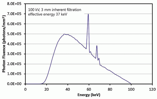
▪ FIGURE 11-1 A typical x-ray spectrum used in radiography, fluoroscopy, and other x-ray imaging systems is illustrated. This is a 100-kV spectrum with 3 mm of inherent aluminum filtration. The area of the spectrum normalized to 1 mGy air kerma, and the half-value layer is 3.8 mm of aluminum. The average energy is 50 keV, and the effective energy is 37 keV.
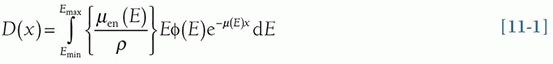
where the photon fluence is φ(E) in #photons/cm2, the mass-energy absorption coefficient is µen(E)/ρ for photons of energy E, ρ is the density of the material, and µ(E) is the linear attenuation coefficient for photons of energy E.
a. The transmitted x-ray fluence for primary photons (Eq. 11-2) is reduced by attenuation (Fig. 11-2) as

▪ FIGURE 11-2 The transmitted x-ray beam shows the approximately exponential attenuation versus tissue depth for the x-ray spectrum illustrated in Figure 11-1. The red filled circles indicate the remaining transmission fraction of a monoenergetic x-ray beam comprised of 37-keV x-ray photons, the monoenergetic approximation to the attenuation curve of the 100-kV polyenergetic spectrum, as a function of depth. As the beam passes through tissue, photons interact by the photoelectric effect, Rayleigh scatter, and Compton scatter interactions and are fractionally eliminated from the primary beam as shown by the attenuated curve. The data show only the attenuation of the primary x-ray beam, assuming a parallel, nondivergent beam geometry.
b. The intensity of the beam is reduced independent of attenuation by the inverse square law, as x-rays are emitted from a point source (the focal spot) with a diverging beam (Fig. 11-3)
3. Generation of x-ray scatter: the complex geometry of x-ray scatter and other factors requires the use of computer-based Monte Carlo techniques to track the passage of primary and scatter photons.
 ▪ FIGURE 11-3 Because the x-ray beam is emitted from essentially a point source, the inverse square law also reduces the intensity of the beam as a function of tissue depth, even if there was no tissue present. This curve assumes a specific x-ray beam geometry, where A = SSD = 68 cm, and B = 30 cm (see inset figure). |
11.2 MONTE CARLO SIMULATION
All modern x-ray dosimetry relies extensively on Monte Carlo simulation. Sophisticated computer programs and algorithms track simulated x-ray photons as they are incident on the patient and in the tissue, photon by photon. Photons that do not interact with the patient, the primary photons, are those used to form the image. The vast majority of photons that do interact with the tissue (greater than 90% of the total) deposit dose through the photoelectric effect and Compton scattering. The statistical probabilities of the interactions and noninteractions followed for billions of photons derived from a polyenergetic spectrum provide a way to determine the dose to the skin and various organs in the body as explained in this section.
1. Computing the random walk of each x-ray photon
a. Each incident x-ray from a bremsstrahlung spectrum is followed through stochastic processes and random number generators (Fig. 11-4).
b. Included are attenuation and geometry-dependent inverse square law processes described in Section 11.1, as well as photoelectric absorption and Compton scatter probabilities for each x-ray photon history.
c. The simulation loops over the energies (e.g., in 1 keV steps) in the filtered bremsstrahlung spectrum.
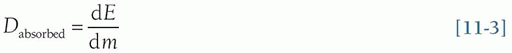
2. The quantity absorbed dose (Eq. 11-3) is the energy deposited (dE) by ionizing radiation per unit mass (dm):
3. The probability of dose deposition depends on x-ray photon energy and the tissue composition (fat, soft tissue, bone) at a specified depth to determine the likelihood of interaction and amount of deposited dose.
a. The photoelectric absorption interaction results in local deposition of most or all of the photon energy.
b. The Compton scatter interaction deposits a fraction of the incident photon dose, and a scattered photon continues on the random walk, emitted at an angle dependent on its energy and the tissue.
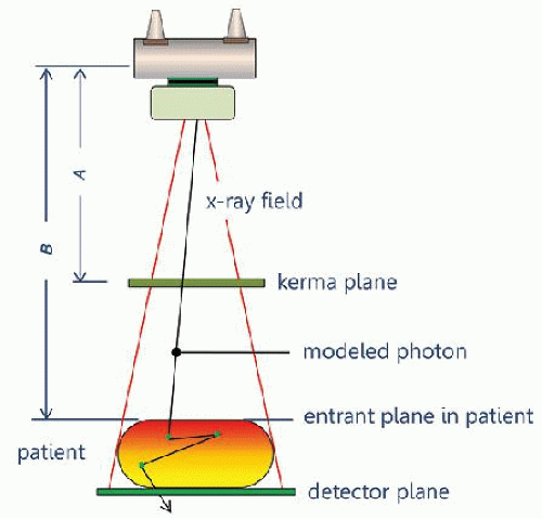
▪ FIGURE 11-4 A typical design for Monte Carlo simulation of dose deposition is illustrated. The simulated (virtual) x-ray beam is emitted from a point source and is collimated onto a detector plane. X-ray interactions are computed in a virtual patient, where the dose deposition and its distribution are tallied. The air kerma passing through the kerma plane is recorded, and the radiation dose in the patient is also tallied. This geometry can then be used to define a coefficient, which is the ratio of patient dose to incident air kerma. More specific anatomical geometry can also tally dose to specific organs and other interaction sites of interest.
4. Normalization point for entrance air kerma
a. Radiography and fluoroscopy: air kerma at the surface of the patient
b. Computed tomography: air kerma at the center of rotation (the isocenter)
5. Mathematical phantoms
a. Simple geometrical phantoms to detailed anatomical models (Fig. 11-5) are used to simulate the body.
b. Anatomical models are segmented into relatively large (2 × 2 × 2 mm voxels) for use in simulations.
 ▪ FIGURE 11-5 A. Historically, Monte Carlo studies made use of anatomical models defined by simple geometrical shapes; here, the Medical Internal Radiation Dose (MIRD) phantom is illustrated. B. The power of modern computers combined with the availability of high-resolution anatomical data from CT scans have allowed Monte Carlo simulations to be performed with very detailed anatomical models. |
11.3 THE PHYSICS OF X-RAY DOSE DEPOSITION
1. X-ray interactions with electrons deposit dose to tissue
a. Photoelectric effect and Compton scatter ionize atoms/molecules at the site of interaction
b. An ejected electron further interacts with tissue in a very small local volume.
c. Electron collision with other electrons (called secondary electrons or “delta rays”) imparts energy.
d. Energy deposition can cause chemical changes (e.g., creation of hydroxyl radicals) that can damage DNA.
2. Kerma
a. Kerma—“Kinetic energy released in matter.”
c. X-ray interactions transfer energy to electrons—the absorbed energy is the difference of the energy transferred (Etr) and the energy radiated (Er) out of the volume (Fig. 11-7) as given by Equation 11-4.

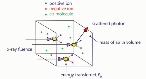
▪ FIGURE 11-6 The basic concept of air kerma is illustrated. X-rays are incident upon a small volume of air and ionize air atoms producing ion pairs as defined in the figure. With these interactions, x-ray photons transfer their energy to the ion pair, resulting in the kinetic energy of these charged particles. When a Compton scattering event takes place, the scattered photon leaves the volume of interest. The air kerma (kinetic energy released in matter) is the energy transferred to charged particles, divided by the mass of the air in the measurement volume.
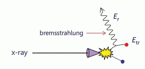
▪ FIGURE 11-7 When an x-ray interacts with an atom or molecule that transfers energy to an ion pair (Etr), subsequent interactions between an energetic electron and other atoms in the interaction volume can result in deceleration of the electron, producing bremsstrahlung radiation (Er: radiated energy). When the bremsstrahlung x-ray leaves the measurement volume, the absorbed energy (Een) is given by: Een = Etr – Er.
3. Absorbed dose in a medium (Fig. 11-8)
 ▪ FIGURE 11-8 When x-ray photons are incident upon the measurement volume (x-ray fluence density), energy is initially transferred (Etr), and some energy may be radiated away (as shown in Fig. 11-7). The energy remaining, Een, divided by the mass of the volume represents the absorbed dose. The volume of interest in this figure could be filled with air, and hence, the dose would be the air dose; however, this can also be a small volume of tissue, corresponding to the absorbed dose in tissue. |
11.4 DOSE METRICS
There are a number of metrics that describe dose in different ways
1. Entrance skin air kerma (ESAK)
a. The amount of radiation incident on the surface of the patient (formerly entrance skin exposure [ESE]).
b. ESAK is an appropriate metric for radiographic, mammographic, and fluoroscopic procedures.
c. The ESAK value is estimated and derived from known output characteristics and geometry at the skin surface and is equal to the air kerma, Kair, at that point.
(i) Value is “free-in-air”—meaning that there is no influence of scatter from any medium in proximity.
d. For diagnostic radiology energies, the air kerma, Kair, approximates the dose to air, Dair: Kair ≈ Dair
2. Entrance skin dose
a. Radiation dose imparted to the initial layers of skin.
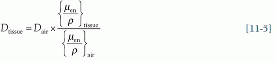
b. The entrance skin dose includes (i) the dose in air, Dair (without backscatter); (ii) dose deposited to the skin by photons backscattered from the tissue volume; and (iii) the ratio of the tissue to air mass-energy attenuation coefficients relating the dose to tissue, Dtissue, to that measured in air, Dair.
(i) The ESAK is equivalent to the dose in air, Dair, without backscattered radiation.
(ii) Backscattered radiation contributes to the dose at the entrance surface—the backscatter factor is variable, dependent on tissue thickness and field size irradiated, ranging from approximately 1.1 to approximately 1.5.
(iii) The ratio of the tissue to air mass-energy attenuation coefficients for a small irradiated area accounts for an increase to the dose in tissue, where Dtissue [all equal to] 1.09 Dair (Eq. 11-5).
3. Absorbed dose
a. Considered to be the fundamental concept of radiation dose.
b. Absorbed dose is the energy absorbed per unit mass (Eq. 11-3).
c. With energy expressed in joules and mass expressed in kilograms, the unit is the gray (Gy); 1 Gy = 1 J/kg.
d. Absorbed dose is specified at a specific point—the dose nearly always varies with position in the patient.
e. Dose is often misinterpreted as a metric directly related to “risk” as described below:
(i) Specification of the total mass of tissue that receives a given absorbed dose can have widely different impacts in terms of risk: for example, 10 Gy to a 20-mg finger versus average dose of 10 mGy to a 20-kg abdomen.
(ii) In the example, the finger and the abdomen receive the same absorbed dose, but the same risk?
(iii) Deposition of dose into organs or tissues affects the risk (see effective dose description, part 6 below).
f. Absorbed dose or just “dose” is the gold standard measurement describing one or more radiation exposure events.
4. Mean glandular dose (also known as average glandular dose)
a. The mean glandular dose (MGD) is the dose metric for describing dose to the breast tissue, composed of fibroglandular, adipose (fat), and skin tissues—methods to determine MGD are explained in Chapter 8.
b. Radiosensitivity of glandular tissue is far greater than skin or adipose tissue.
c. MGD is the standard metric for computing dose in the breast.
5. Organ dose
a. Metrics
(i) Average (mean) dose delivered to the specific organ of interest
(ii) For paired organs (e.g., kidneys or breasts), if a targeted examination deposits dose in only one (e.g., 0.2 mGy to the left kidney), the average dose to both kidneys for the procedure would be 0.1 mGy.
(iii) Implicit assumption is that the stochastic risk is the same whether one half of the organ receives all of the radiation or if the radiation dose was evenly distributed throughout the entire organ.
b. Anthropomorphic phantoms
(i) Organ doses from x-ray exposures in anthropomorphic phantoms can be estimated with Monte Carlo techniques (for further details, see Fig. 11-5, and textbook Pg. 418, Fig. 11-9)
(ii) A balance between accuracy and simulation efficiency for organ dose comes in the form of “hybrid modeling,” which combines analytical and Monte Carlo simulation methods on stylized or computational human phantoms ranging from the newborn to (male and female) adults
c. No one dose metric can do it all.
(i) A tally of organ doses represents the comprehensive assessment of radiation dose from imaging.
(ii) There is no single metric that can quantify “dose” and the corresponding radiosensitivity of an organ.
(iii) Different radiation types (x-rays, gamma rays, electrons, protons, alpha particles) can deposit dose quite differently in tissues, and increase the probability of stochastic effects like cancer for the same absorbed dose; the dose metric called equivalent dose accounts for differences in the type of radiation.
6. Equivalent dose
a. Accounts for the biological damage to tissues based upon the consequence of linear energy transfer (LET) deposition of different radiation types through the use of weighting factors, wR (Eq. 11-6).
b. Sparsely ionizing low LET radiations (e.g., x-rays, γ-rays, electrons) are assigned wR = 1.
c. Densely ionizing high LET radiations (e.g., protons, alpha particles) are assigned wR greater than 1; for example, wR = 20 for alpha particles (See Chapter 3, Pg. 65-66, and Table 3-4 in the textbook).
d. The quantity equivalent dose, H, is

e. Note: for x-rays, the equivalent dose is numerically equal to the absorbed dose, but they are different quantities—unit of equivalent dose is the sievert (Sv), and unit of absorbed dose is the gray (Gy).
7. Effective dose, E
a. Like H, E is a calculated value that is not really a dose in the physical sense. E is a radiation protection term that provides a single value metric for the cumulative long-term potential for harm (detriment) to a population for exposures to different areas of the body.
b. Originally proposed for assessment of environmental and industrial exposure to radiation workers.
c. Organs that do not receive dose do not contribute to E.
d. Incorporates an approximation of organ sensitivities and assigns a tissue weighting factor, wT.
(i) For uniform whole-body irradiation, the total tissue weighting is 1.0—thus, the individual organ wT sum to 1.0.
(ii) A proportion of the total is the wT of the organs, assigned according to organ-tissue sensitivity, (mostly radiogenic cancer).
e. Quantifying effective dose, E, is a two-step process.
(i) Organ absorbed dose, D (Gy), is converted to organ equivalent dose, HT (Sv), using Equation 11-6.
(ii) The effective dose E (units of Sv) is calculated using Equation 11-7 for all organs irradiated T, as the sum over T of the product of wT and the corresponding organ equivalent dose HT as:

TABLE 11-1 TISSUE WEIGHTING FACTORS (WT) FOR VARIOUS TISSUES AND ORGANS (ICRP 103)
TISSUE
WT
Bone marrow, breast, colon, lung, stomach, remainder
0.12
Gonads
0.08
Bladder, esophagus, liver, thyroid
0.04
Brain, bone surface, salivary glands, skin
0.01
f. Strengths of effective dose, E
(i) E takes into consideration partial body exposure.
(iii) E provides a single value metric for the long-term potential for harm (detriment) to a population for multiple exposures to different areas of the body.
(iv) E can be used to make numerical comparisons to radiation doses associated with medical imaging procedures in a more understandable context for patients and healthcare workers—for example, comparison of annual background radiation of 3.1 mSv at sea level to a head CT effective dose of 2.5 mSv.
g. Weaknesses of effective dose
(i) As defined by the ICRP, E was never meant and should not be used as a risk-related metric for a specific person or population that differs from the population used to define the weighting factors. Unfortunately, all too often, E has been popularized as a quantitative measure of individual future cancer risk, a use for which it was never intended.
(ii) As a risk metric, E does not take into consideration patient-specific factors such as health status, clinical indication, patient sex, patient age—all factors that must be considered when evaluating potential risks against the benefits of a particular imaging procedure,
h. E is useful in comparing imaging modality doses (e.g., CT versus radiography) to the same patient population.
11.5 RADIATION DOSE IN PROJECTION RADIOGRAPHY
1. X-ray system radiation output levels
a. Measurable normalized values of radiation output (Fig. 11-9).
b. Information is typically provided by annual testing of radiographic equipment.
c. Air kerma (mGy) per 100 mAs at 100 cm as a function of x-ray tube kV (and any added filtration).
a. Distance: source to skin distance (SSD) and source to image distance (SID) (Fig. 11-10)
b. Inverse square law: relates measured x-ray tube output air kerma at 100 cm to x SSD (cm)
c. Tube current-time product (mAs): relates mAs used for the examination, x, to 100 mAs measured output
d. Determine air kerma from output curve graph (Fig. 11-9) for the kV used in the examination, AK (kV)
e. Calculate the ESAK as the product of C1, C2, and AK (kV)

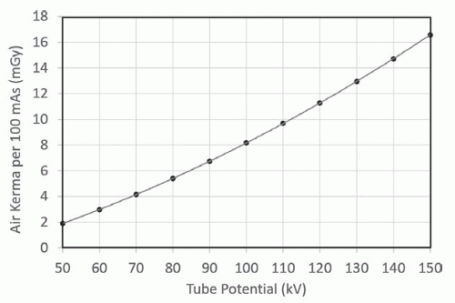
▪ FIGURE 11-9 Measures of air kerma for given x-ray tube potentials (kV) for various tube current-time products (mAs) are performed as a part of annual consistency testing. These data were computed to a distance of 100 cm from the x-ray source. Notice the slight curvature of the data, indicating a (kV)n dependency on x-ray output, where n is greater than 1. F. 11-10
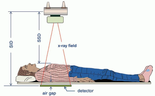
▪ FIGURE 11-10 The imaging geometry for an AP radiograph. For most tabletop radiographic imaging protocols, the source to image distance (SID) is typically 100 cm. The air gap between the bottom of the patient and the top of the detector can be estimated and is typically between 2 and 5 cm. Estimating patient thickness then allows the source to skin distance (SSD) to be estimated. F. 11-12
3. Estimating effective dose
a. Tabular data are available for computing organ doses and effective doses from ESAK for specific examinations.
(i) See textbook, Page 425, Table 11-3: Effective dose per entrance surface dose (mSv/mGy) conversion factors for various kV, filters, and radiographic projections
b. Digital radiography systems provide kerma area product (KAP) measurements directly; this metric is often called dose area product (DAP)
(i) The KAP, sometimes indicated as PKA, is equal to the product of the cross-sectional area of the x-ray beam and air kerma exiting collimator and provides a dose metric that is constant with distance.
(ii) Air kerma at a specific distance can be determined by indicated KAP divided by the beam area projected at that distance (e.g., onto the patient at the SSD).
(iii) Total energy imparted to the patient is proportional to KAP and also to effective dose.
(iv) Monte Carlo routines for projection radiography can be used to estimate effective dose for specific projections by knowing the acquisition technique factors (kV, mAs, tube filtration/half-value layer, field area projected onto the anthropomorphic phantom).
(v) A graphic relationship of KAP to effective dose conversion factor can be determined as the slope of the linear regression fit of data points for different patients (Fig. 11-11).
 ▪ FIGURE 11-11 The kerma area product (KAP), also referred to as the dose area product (DAP) in the DICOM header, is a metric available on modern digital radiography systems. A. An anterior-posterior (AP) projection of the pelvis in a thin patient, with a measured KAP of 2.61 dGy-cm2. (Note, dGy-cm2 is the standard DICOM unit for KAP, not the more commonly used, but equivalent unit of mGy-cm2.) B. Plot of the calculated effective dose versus indicated KAP for a range of patient sizes using x-ray acquisitions with automatic exposure control. The linear regression fit gives the slope (mSv/dGy-cm2) and offset, which is used to estimate effective dose directly from the KAP for any similar examination. For the patient radiograph shown in (A), the effective dose is estimated to be 0.046 mSv (0.0118 + 0.0133 × 2.606).  F. 11-13 F. 11-13 |
11.6 RADIATION DOSE IN FLUOROSCOPY
1. Considerations relative to radiography
a. Acquisitions vary over an extended time, with variations in tube current.
b. Geometrically, fluoroscopy changes with interactive movements for patient repositioning.
c. Several magnification modes can be selected that change air kerma rate and FOV.
d. The operator can change the beam projection angle throughout the procedure.
e. SID often changes throughout the procedure with table height and detector adjustments.
f. FOV collimation can be circular, square, or rectangular.
g. kV and filtration are interactive, dependent on fluoro mode used (e.g., low, medium, high dose).
2. Automatic exposure (air kerma) rate control (AERC)
a. AERC adjusts the kV and mA to achieve an acceptable image as needed by the examination.
b. Adjustments include selection of low dose, medium dose, or high contrast as required.
c. Measurements in the field with various attenuator thicknesses can validate operation (Fig. 11-12).
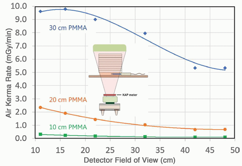
▪ FIGURE 11-12 Virtually all modern fluoroscopic systems work in automatic exposure rate control mode, and therefore, characterization of the output of the system needs to embrace this. The air kerma rate is shown as a function of the detector field of view, for three thicknesses of polymethyl methacrylate (PMMA), a tissue surrogate. For calculation of patient dose in fluoroscopy using the data shown in the figure, the medical physicist also needs to know (for each touch of the fluoroscopic pedal) the patient thickness and the detector field of view. For patient thicknesses that are substantially different from the three shown (10, 20, and 30 cm) exponential, interpolation can be used at each detector field of view setting. F. 11-14
3. Estimates of radiation dose in fluoroscopy
a. Integrated air kerma at the reference point, Ka,r, and kerma-area product (KAP or PKA) are required.
(i) For interventional systems, Ka,r is 15 cm closer to the x-ray tube from the isocenter of rotation.
(ii) For mobile C-arm fluoroscopy units, Ka,r is determined 30 cm from the detector entrance surface.
b. DICOM Radiation Dose Structured Report (RDSR) provides a recording of each irradiation event with all x-ray output parameters, collimation, geometric orientation, and operation mode.
c. The cumulative Ka,r is a surrogate for estimating peak skin dose for possible tissue reactions and injuries.
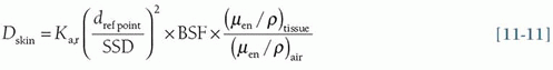
(i) Dose to the skin can be estimated from Ka,r and distance, d, to the reference point from the focal spot to the skin, SSD, by inverse square correction, the backscatter factor (BSF) that ranges from 1.1 to 1.5 dependent on field size and patient thickness, and tissue-to-air ratio of approximately 1.09 in Equation 11-5 above.
(ii) Estimates of peak skin dose (PSD) or Dskin use Ka,r data and beam geometry/orientation from the RDSR data and BSF (Eq. 11-11), as well as attenuation of the table/pad as described in Chapter 9
(iii) A sentinel event as defined by The Joint Commission is an acute PSD of 15,000 mGy (15 Gy) or consecutive studies that exceed 15,000 mGy when summed over a 6-month period.
(iv) “Procedural pause” occurs when Ka,r reaches predetermined limits (e.g., 5,000 mGy, 7,000 mGy, etc.) to identify next steps and as a reminder to spread dose over a large area of the body.
d. The KAP (PKA) allows the determination of energy imparted to the patient and can be used with conversion factors to estimate effective dose (and thereby an estimate of risk) for the fluoro examination
(i) Methods are similar to those described above in Section 11.5.3.b.
(ii) Conversion factors with units of mSv/mGy-cm2 for various procedures are available in the literature.
11.7 RADIATION DOSE IN COMPUTED TOMOGRAPHY
The computed tomography dose index (CTDI) is a metric that considers the unique characteristics of CT, including no well-defined entrant surface, rotation about an isocenter, spatial dependence of beam-shaping filters, and acquisition parameters that impact the delivered dose to the patient. CTDI is not patient dose and does not consider the size of the patient. It does, however, represent a measure of the radiation output of the CT scanner.
1. Computed Tomography Dose Index, CTDI100
a. CTDI100 uses a 100-mm-long “pencil” ionization chamber of approximately 9 mm diameter and approximately 3 cm3 volume with a uniform radiation response along its length.
b. A cylindrical polymethyl methacrylate (PMMA) phantom of 15 cm length is used for measurements.
(i) 16-cm phantom: output measurements to represent adult and pediatric head scans
(ii) 32-cm phantom: output measurements to represent the adult body and a majority of pediatric body scans
(iii) 16-cm phantom: to represent small diameter pediatric body studies by some CT scanner vendors, although many vendors use the large 32-cm-diameter phantom for all pediatric body studies
c. Each phantom has several parallel holes for insertion of the pencil ionization chamber (Fig. 11-13).Related posts:

Stay updated, free articles. Join our Telegram channel

Full access? Get Clinical Tree