. Since often multiple source components2 are active at the same time, the measured magnetic fields and electric potentials represent a superposition of all contributions. Each source component can be characterized by a set of parameters (see below) and by the signals it produces at sensor level. These signals are often termed components of the signal (Donchin 1966; Kayser and Tenke 2005). In the literature on source separation the term “source” is often used synonymously for the signal the source component is producing, whereas in the literature on source reconstruction it is used to describe the parameterized source model.
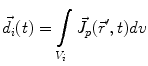
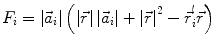
The primary current density  is a spatially continuous function. In order to describe it with a finite vector of parameters, two approaches exist. The discretization approach divides the space into sections, within each of which the current density is replaced by the integral over the volume of that section:
where  denotes the dipole moment typically given in nanoamperemeters [nAm]. The discretization approach is based on the topology of the source space. For example, the entire brain volume can be discretized in hexahedral voxels, or the cortical sheet can be discretized into prisms (triangles representing the cortical surface plus a predefined thickness). In each of these elements, the primary current density is modeled by one current dipole.
is a spatially continuous function. In order to describe it with a finite vector of parameters, two approaches exist. The discretization approach divides the space into sections, within each of which the current density is replaced by the integral over the volume of that section:(1)
denotes the dipole moment typically given in nanoamperemeters [nAm]. The discretization approach is based on the topology of the source space. For example, the entire brain volume can be discretized in hexahedral voxels, or the cortical sheet can be discretized into prisms (triangles representing the cortical surface plus a predefined thickness). In each of these elements, the primary current density is modeled by one current dipole.In many practical applications the primary current density is relatively focal, such that it can be satisfactorily described by a few current dipoles at the centers of activity leading to the multiple dipoles model. The second approach parameterizes the primary current density with the help of a series expansion. The series can also describe extended source configurations centered at the expansion point. Often, the electric potential at the measurement location  expressed by a Taylor series expansion with the origin at position
  :
:
![$$\varphi (\vec{r}) = \frac{1}{4\pi \sigma }\left[ {\frac{m}{{\left| {\vec{r} - \vec{r}'} \right|}} + \frac{{\vec{d}(\vec{r} - \vec{r}')}}{{\left| {\vec{r} - \vec{r}'} \right|^{3} }} + \frac{1}{{\left| {\vec{r} - \vec{r}'} \right|^{3} }}\left( {\frac{3}{{\left| {\vec{r} - \vec{r}'} \right|^{2} }}(\vec{r} - \vec{r}')^{T} \bar{q}(\vec{r} - \vec{r}') - tr(\bar{q})} \right) + \cdots } \right]$$](/wp-content/uploads/2016/04/A272390_1_En_4_Chapter_Equ2.gif)
expressed by a Taylor series expansion with the origin at position :(2)
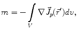
Here, m is the electric monopole moment, which vanishes due to the charge conservation law:
 is the dipole moment according to Eq. (1) and
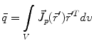
  is the quadrupole tensor:
(3)
is the dipole moment according to Eq. (1) and is the quadrupole tensor:(4)
A truncation of this series, after the dipole term, results in the equivalent current dipole model which represents the entire current density as a point-like current element. Extending this approach to multiple partial volumes yields the same multiple dipoles model, which was derived from the discretization approach above.
The sensor model describes how a sensor transforms a physical quantity into an accessible output. For biomagnetic measurements this typically involves first the transformation of the magnetic flux density into a magnetic flux by integration over the area of a pickup coil. Next this magnetic flux is often combined across several coils in order to suppress far field disturbances. Finally, the magnetic flux is converted into a voltage. Important parameters of this model are the position, orientation, geometrical form, and number of windings of the coils. The exact integration of the flux density over the coil area would be computationally demanding. Thus, often the flux density at the center point of the coil is assumed to represent the constant value over the entire coil area. More accurate approaches involve a weighted average of the flux density at a small number of integration points within the coil area. Magnetic recordings do not require a reference, which is an advantage compared to electric recordings.
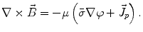
Next we consider the description of the relationship between source parameters and the simulated data at the sensors. Maxwell’s equations are the basis for this transfer function. For most non-invasively measured electric and magnetic bio-signals, frequencies are below 1,000 Hz and the spatial dimension is below 1 m. Consequently, the temporal derivatives in the Maxwell equations can be omitted (Plonsey and Heppner 1967), yielding the quasi-static Maxwell equations that disregard capacitive and inductive effects (Table 1). The free volume charge density is not relevant here, since we consider the electric flow field only, which is uncoupled from the electrostatic field due to the vanishing derivative of D in the quasistatic approximation of Ampère’s law (Table 1). The only remaining relevant material parameter is the electrical conductivity.
Table 1
Full and quasi-static Maxwell equations
Faraday’s law | Amperè’s law | Gauß’s law | Gauß’s law for mag. | Material equations | |
|---|---|---|---|---|---|
Full | 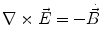 | 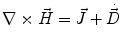 |  |  |    |
Quasi-static |  |  |  |  |
The vectorial state variables comprise the electric field strength  , the magnetic field strength
  , the electric current density
  , the magnetic induction
  and the electric displacement current density
  . The material tensorial parameters are the electrical conductivity
  , the permittivity
  and the permeability
  . The scalar parameter ρ f denotes the free volume charge density
, the magnetic field strength , the electric current density , the magnetic induction and the electric displacement current density . The material tensorial parameters are the electrical conductivity , the permittivity and the permeability . The scalar parameter ρ f denotes the free volume charge densityFrom the definition of the scalar electric potential  (based on the quasi-static law of Faraday) and Ohm’s law
  , one can derive Poisson’s equation (Eq. 5), while the quasi-static law of Ampère allows (under the assumption of a scalar magnetic permeability
  ) for computing the magnetic field from the electric potential (Eq. 6).
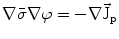
(based on the quasi-static law of Faraday) and Ohm’s law , one can derive Poisson’s equation (Eq. 5), while the quasi-static law of Ampère allows (under the assumption of a scalar magnetic permeability ) for computing the magnetic field from the electric potential (Eq. 6).(5)
(6)
This leads to expressions for the electric potential φ and the magnetic induction  at position
  , arising from N dipoles at positions
  with moments
  , in an infinite volume with homogeneous and isotropic conductivity.
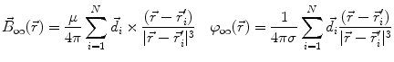
at position , arising from N dipoles at positions with moments , in an infinite volume with homogeneous and isotropic conductivity.(7)
These equations, however, do not provide an acceptable solution for the situation in real biological tissue as they do not take into account the effects of conductivity inhomogeneities. If very simplifying assumptions about the distribution of conductivities are made, analytical or semi-analytical solutions can be used. The human head can be modeled with the help of a series of spherical or ellipsoidal layers (Cuffin and Cohen 1977; Sarvas 1987; de Munck 1988, 1989; Kariotou 2004; Giapalaki and Kariotou 2006). Such models allow for easy computations, but can yield significant errors (Cuffin and Cohen 1977).
More realistic conductivity profiles can be modeled using numerical methods. These methods can be classified into differential and integral methods depending on whether derivatives or integrals are to be approximated. Additionally, methods can be classified according to their basic assumptions and simplifications. A crucial property of the head is the fact that a relatively low-conducting skull encloses the relatively well-conducting brain. In turn, the skull is surrounded by a relatively well-conducting remainder of the head (scalp, muscles, eyes, etc.). This leads to the compartment assumption. Typically, 3 compartments with homogeneous and isotropic conductivity are defined: scalp, skull and brain. The brain compartment subsumes all tissues inside the skull. The skull compartment includes both compact and spongy bone. The scalp compartment summarizes all tissues outside the skull. The compartment approach necessitates the use of an integral-based method.
Alternatively, the compartment assumption can be replaced by a 3D volume discretization. Here, the volume is divided into small elements. The size and number of elements governs the achievable accuracy and is limited by computational resources. Volume discretization approaches are usually treated with differential methods.
The boundary element method (BEM) is an integral method based on the compartment assumption (Barnard et al. 1967a, b; Geselowitz 1967, 1970; Sarvas 1987; Hämäläinen and Sarvas 1989; Stenroos et al. 2007). An alternative approach is the multiple multipole method (MMP) (Haueisen et al. 1996). Here, multipole expansions are used to describe the neuroelectromagnetic field and the expansion coefficients may be computed based on a matching of the boundary conditions at a set of boundary points representing the major conductivity jumps. For modeling the 3D or anisotropic conductivity profile of the head, the finite element method (FEM) (Witwer et al. 1972; Haueisen et al. 1995; Wolters et al. 2004; Hallez et al. 2005) or the finite difference method (FDM) (Witwer et al. 1972; Haueisen et al. 1995; Wolters et al. 2004; Hallez et al. 2005) can be used. Both are differential methods. The entire volume is discretized into small elements and each volume element is assigned a separate conductivity tensor. While FDM is easier to implement, FEM allows for a smoother geometry description of conductivity boundaries. For a review including the FEM and FDM see e.g. (Hallez et al. 2007).
In the following, we will treat analytical methods, BEM, and FEM in more detail, since these methods are most frequently used. Figure 1 shows an example model for BEM and FEM.
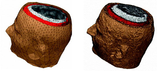
Fig. 1
Examples for head models. Left boundary element model with the most important conductivity boundaries (inner and outer skull surface, outer surface of the head) described by triangular meshes. Right finite element model built with tetrahedral elements. Colors represent tissue types
2 Analytical and Semi-Analytical Methods
In order to obtain analytical or semi-analytical formulations of the forward problem, the geometry of the head and the conductivity distribution have to be described in terms of simple shapes, such as concentric spherical or ellipsoidal shells. In the simplest case, the volume conductor is assumed to be a sphere, which is more or less adapted to the actual head geometry. Under this assumption, for MEG it can be shown that the predicted magnetic field outside the head depends solely on the origin of the sphere as well as the positions and orientations of the sources and the sensors. The conductivity profile including the outer radius, as long as it is spherically symmetric, plays no role. According to Sarvas (1987), the magnetic induction  at sensor position
  due to N dipoles at positions
  with dipole moments
  (i = 1…N) is computed as follows:


at sensor position due to N dipoles at positions with dipole moments (i = 1…N) is computed as follows:(8)
(9)
(10)
(11)
Another important property of this volume conductor model can be seen from the formula above: a dipole with radial orientation does not contribute to the measured field. Its effect is completely compensated for by the Ohmic return currents.
In contrast, the predicted EEG on the surface of a spherical volume conductor does depend on sources of all orientations, as well as on the conductivities and radii of the different tissue layers. A semi-analytical solution based on Legendre polynomials is given by de Munck (1989). It allows for the inclusion of tissue compartments with different conductivities, bounded by concentric spherical surfaces. It even allows for a simple form of tissue anisotropy, namely the distinction between radial and tangential conductivities.
Although spherical models reflect the basic geometric properties of the head, such as its round shape and the concentric arrangement of the tissue layers, the deviations from the real head shape may lead to substantial errors (Cuffin and Cohen 1977). There are a number of possibilities to improve this situation without giving up the advantages of an analytical solution. One option is the use of ellipsoidal instead of spherical shells, as proposed, for example, by Fieseler (Fieseler 1999) and Kariotou (Kariotou 2004; Giapalaki and Kariotou 2006).
Alternatively, one can use a separate spherical volume conductor model for each sensor. One way to find these local spheres is to fit them locally to a patch of the head (or brain) surface near the respective sensor (Ilmoniemi 1985; Lütkenhöner et al. 1990). This assumes that the description of the tissue boundaries in the immediate vicinity of the respective sensor is most crucial for the accuracy of the forward computation. A more principled, but also computationally more expensive, way to find the best spherical models on a sensor-to-sensor basis was proposed by Huang et al. (1999). They first used a realistic 3-shell boundary element model (see below) to compute solutions in each sensor for a large number of dipoles located in the entire brain (i.e., a leadfield computation, see below). Then, for each sensor, the solutions for the same dipoles were computed using a spherical head model, and the parameters of that spherical model were optimized such that the difference between the boundary element method solution and the spherical solution became minimum. For MEG, a single-compartment boundary element model can be used alternatively. The resulting spheres can then be used to calculate forward solutions for arbitrary dipoles. In principle, this method can be seen as a sophisticated way for interpolating leadfields computed using numerical methods, such as BEM. For a review and evaluation of different methods using multiple spheres, see Lalancette et al. (2011).
Finally, Nolte (2003) proposed an approach, where the solution for a spherical volume conductor is corrected by a superposition of basis functions constructed from spherical harmonics and fitted to the boundary conditions. It can be shown that this approach yields good approximations for non-spherical volume conductors such as the prolate spheroid (Nolte 2003) and even for realistically shaped volume conductors (Stenroos et al. 2012).
3 Numerical Methods
3.1 Boundary Element Method
The BEM is an important and popular field calculation method used in biomagnetism. It can describe the head as an isotropic and piecewise homogeneous volume conductor of realistic shape. In practice, the compartments are designed such that their boundaries represent the most prominent conductivity jumps in the head. These are most often the head surface as well as the outer and inner bounds of the skull. For MEG, the volume currents outside the interior of the skull contribute relatively little to the measurements and therefore the respective compartments (skull, scalp) are often neglected (Hämäläinen and Sarvas 1989). However, it was recently shown that the inclusion of the skull and scalp compartments allows for a relevant improvement in accuracy (Stenroos et al. 2012).
Mathematically, the solution is derived from Poisson’s equation (Eq. 5) and the appropriate Cauchy boundary conditions: (1) the potential has to be continuous across the boundary:  , and (2) the perpendicular component of the current has to be continuous across the boundary3:
 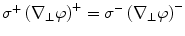 , where the superscripts ()+ and ()−
 Decoding and Brain Machine Interfaces Based on Electromagnetic Oscillatory Activities: A Challenge for MEG
Neuroscience: A New Frontier for Magnetoencephalography?
Decoding and Brain Machine Interfaces Based on Electromagnetic Oscillatory Activities: A Challenge for MEG
Neuroscience: A New Frontier for Magnetoencephalography?
 Integration
 Imaged Pathways of Stuttering
 Current Imaging with Ultra-Low-Field NMR Techniques
 Concurrent EEG and fMRI Intrinsic Networks


, and (2) the perpendicular component of the current has to be continuous across the boundary3: , where the superscripts ()+ and ()−
Related posts:
Decoding and Brain Machine Interfaces Based on Electromagnetic Oscillatory Activities: A Challenge for MEG
Neuroscience: A New Frontier for Magnetoencephalography?
Integration
Imaged Pathways of Stuttering
Stay updated, free articles. Join our Telegram channel
Full access? Get Clinical Tree
