MR Angiography
Introduction
In this chapter, we will discuss the topic of MR angiography (MRA). As in the last chapter, MRA may at first appear very complicated, but we’ll try to present the major concepts in a simplified fashion. There are three main MRA techniques:
CE (contrast-enhanced) MRA
TOF and PC techniques can be performed using two-dimensional Fourier transform (2DFT) or three-dimensional FT (3DFT). CE MRA is performed with the 3D technique. Thus, there are a total of five different methods:
Each of these techniques lends itself to a different type of clinical application.
TOF MRA
TOF MRA is based on flow-related enhancement (FRE; discussed in the previous chapter) in a 2D or 3D gradient-echo (GRE) technique. (Remember that in GRE imaging, TOF losses do not play an important role.) Usually, flow compensation is used perpendicular to the vessel lumen.
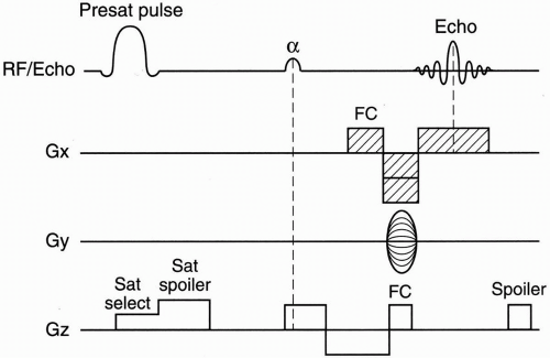
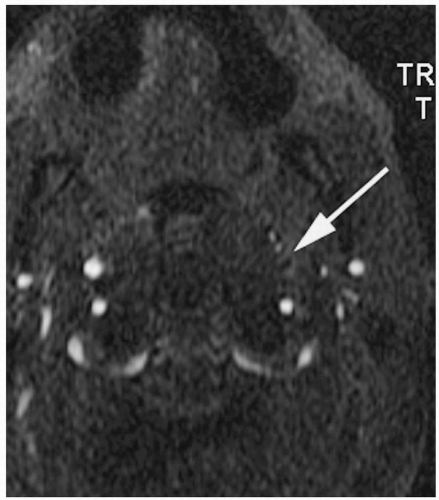
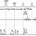
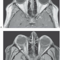
2D–TOF MRA. Figure 27-1 depicts a typical pulse sequence for 2D–TOF MRA. A presat (presaturation) pulse is applied above or below each slice to eliminate the signal from vessels flowing in the opposite direction. Usually a short TR (about 50 msec), a moderate flip angle (45° to 60°), and a short TE (a few millisecond) are used. An example is seen in Figure 27-2.
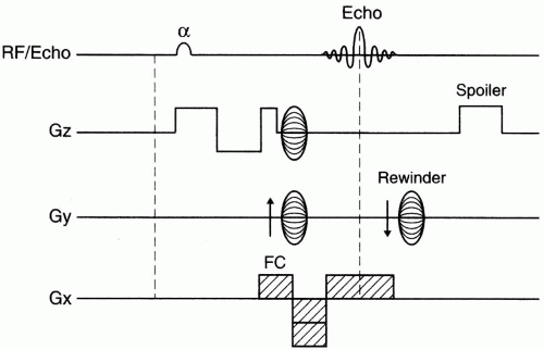
3D–TOF MRA. Figure 27-3 depicts a pulse sequence diagram (PSD) for a 3D–TOF MRA. Here, a slab of several centimeters (usually about 5 cm) is obtained that contains up to 60 slices.
Advantages of 2D-TOF MRA
Faster scanning
Maximized FRE because each slice is an entry slice
Disadvantages of 2D-TOF MRA
In plane saturation effects (discussed later)
Advantages of 3D-TOF MRA
Higher signal-to-noise ratio (SNR) because signal is acquired from a larger volume
Improved spatial resolution
PC MRA
PC MRA is based on the fact that the phase gain of flowing blood through a gradient is proportional to its velocity (assuming constant velocity). We saw in the previous chapter that phase (φ) and velocity (v) are related by φ = ∫ωdt = ∫(γGvt)dt = 1/2γGvt2 Therefore, knowing the phase at any point in time allows us to calculate the velocity.
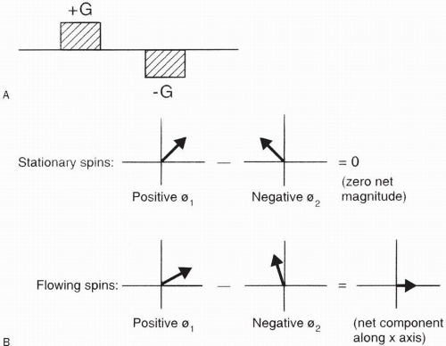
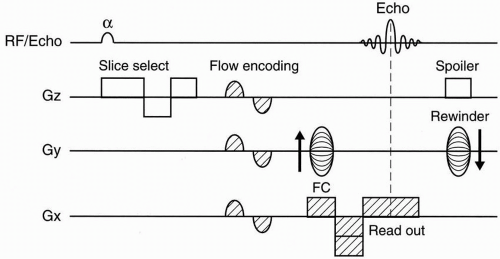
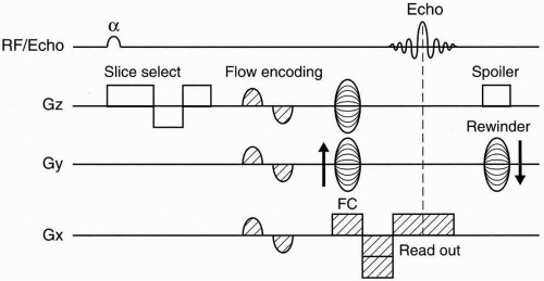
The most common method to employ PC MRA is by the use of a bipolar gradient (Fig. 27-4A). This process is called flow encoding. Because the two lobes in this bipolar gradient have equal area, no net phase change is observed by stationary tissues (Fig. 27-4A). However, flowing blood will experience a net phase shift proportional to its velocity (assuming a constant flow velocity) (Fig. 27-4B). This is how flow is distinguished from stationary tissue in PC MRA. Figures 27-5 and 27-6 illustrate the PSDs for 2D–PC and 3D–PC MRA, respectively.
Question: What are the “magnitude” image and the “phase” image?
Answer: In PC MRA, you not only get an image of the blood vessels (magnitude image); you also get an image that shows you the direction of flow (phase map). The phase image would tell you whether the flow is right-left, superior-inferior, or anterior-posterior. An example is determination of hepatofugal versus
hepatopedal flow in the portal vein of a patient with cirrhosis.
hepatopedal flow in the portal vein of a patient with cirrhosis.
 |
 |
Question: What is VENC?
Answer: VENC stands for velocity encoding. It is a parameter that is selected by the MR operator when using PC MRA. VENC represents the maximum velocity present in the imaging volume. Any velocity greater than VENC will be aliased according to the following formula: Aliased velocity = VENC − actual velocity
For instance, if VENC = 30 cm/sec, then a vessel with a flow velocity of 40 cm/sec will be represented as a flow of v = 30 − 40 = −10 cm/sec that is, a flow of 10 cm/sec in the opposite direction (Fig. 27-7). A smaller VENC is more sensitive to slow flow (venous flow) and to smaller branches but causes more rapid (arterial) flow to get aliased. A larger VENC is more appropriate for arterial flow. Sometimes you may image the same thing with two different VENCs—a small VENC and a large VENC—to image all the flow components accurately (an example is imaging an AVM or an aneurysm).
For instance, if VENC = 30 cm/sec, then a vessel with a flow velocity of 40 cm/sec will be represented as a flow of v = 30 − 40 = −10 cm/sec that is, a flow of 10 cm/sec in the opposite direction (Fig. 27-7). A smaller VENC is more sensitive to slow flow (venous flow) and to smaller branches but causes more rapid (arterial) flow to get aliased. A larger VENC is more appropriate for arterial flow. Sometimes you may image the same thing with two different VENCs—a small VENC and a large VENC—to image all the flow components accurately (an example is imaging an AVM or an aneurysm).
Advantages of PC MRA
The capability to generate magnitude and phase images
Superior background suppression
Less sensitive to intravoxel dephasing or saturation effects
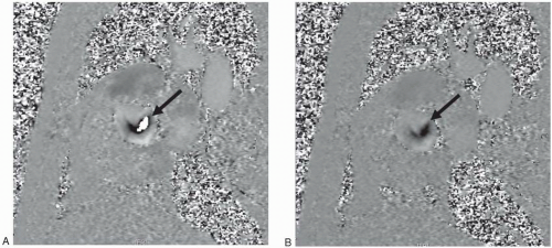 Figure 27-7. Two phase contrast images (phase maps) through the root of the aorta in a patient with aortic stenosis. A: VENC = 150 cm/sec; B: VENC = 300 cm/sec. Note in (A) the bright central signal (arrow) that may indicate regurgitant flow; however, the signal is surrounded by darker signal with abrupt transition from black pixel to white pixel diagnostic of aliasing. Increasing the VENC in (B) eliminated the aliasing. No bright signal indicative of regurgitation was observed and an accurate maximal velocity determination was now possible. |
Disadvantages of PC MRA
Takes longer to do
More sensitive to signal losses caused by turbulence and by dephasing on vessel turns (e.g., carotid siphon)
The need to guess the maximum flow velocity in order to select an optimum VENC
2D- versus 3D-PC MRA
2D techniques are faster
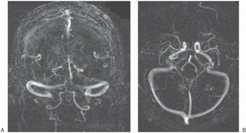
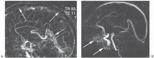
Examples of magnitude phase contrast images are seen in Figures 27-8 through 27-10.
CE MRA
Related posts:
Stay updated, free articles. Join our Telegram channel

Full access? Get Clinical Tree


