Magnetic resonance (MR) perfusion imaging offers the potential for measuring brain perfusion in acute stroke patients, at a time when treatment decisions based on these measurements may affect outcomes dramatically. Rapid advancements in both acute stroke therapy and perfusion imaging techniques have resulted in continuing redefinition of the role that perfusion imaging should play in patient management. This review discusses the basic pathophysiology of acute stroke, the utility of different kinds of perfusion images, and research on the continually evolving role of MR perfusion imaging in acute stroke care.
When magnetic resonance (MR) imaging–based techniques for studying brain perfusion were developed in the 1980s and 1990s, one of the first pathologic conditions to which they were applied was ischemic stroke, a disease that is caused fundamentally by impaired perfusion. Like the positron emission tomography (PET) and single-photon emission computed tomography (SPECT)-based methods that preceded it, MR perfusion imaging of acute stroke patients offered a window into a rapidly evolving disease process, in which changes in tissue perfusion may have dramatic effects on patient outcomes. MR-based perfusion-weighted imaging allowed perfusion measurements to be obtained more quickly than with PET or SPECT, and with scanners that were more widely available.
Interest in imaging perfusion rapidly was spurred by the US Food and Drug Administration’s 1996 approval of intravenous tissue plasminogen activator (tPA), a thrombolytic drug whose purpose is restore brain perfusion, but which was approved for use only in those very few acute stroke patients who can be treated within 3 hours of symptom onset. Because tPA offers both the potential for life-saving rescue of underperfused tissue and the risk of catastrophic intracranial hemorrhage, the most active focus of research on MR perfusion imaging in acute stroke has been its potential application in refining the selection of patients for thrombolysis. However, perfusion imaging also has other potential roles in ischemic cerebrovascular disease, including establishing diagnosis, predicting prognosis, and guiding nonthrombolytic therapies designed to maintain cerebral perfusion.
Before addressing MR perfusion imaging’s potential uses in these roles, this review first discusses the ways in which the various perfusion parameters that can be measured by perfusion imaging vary under different hemodynamic conditions. The following section presents the computational techniques that are used to create the various kinds of clinically used MR perfusion images. Although the details of these techniques and the artifacts that they may create are often overlooked in discussions of perfusion imaging, understanding them is essential to integrating the results of past research on MR perfusion imaging, and to using perfusion imaging in patient care.
The hemodynamics of ischemic stroke
The changes in perfusion that occur in acute stroke are driven fundamentally by global and/or regional changes in cerebral perfusion pressure (CPP). CPP is the difference between mean arterial pressure and venous pressure, the latter of which is usually equal to intracranial pressure. The cerebral vasculature responds to small reductions in CPP by dilating small arteries, thereby reducing cerebrovascular resistance, and successfully maintaining normal cerebral blood flow (CBF) over a wide range of perfusion pressures. This vasodilatory response results in an increase in cerebral blood volume (CBV), which is the volume of the intravascular space within a particular volume of brain tissue, such as that within a single image voxel. The increase in CBV may be subtle and difficult to detect in MR perfusion images. Vasodilation also results in an increase in mean transit time (MTT), which is the average amount of time that red blood cells spend within a particular volume of tissue. CBF, CBV, and MTT are related via the central volume theorem :
When CPP drops below the threshold at which the brain maintains autoregulation, the compensatory vasodilatory response is overwhelmed. CBF begins to decrease, and becomes pressure-dependent, that is, further reductions in CPP lead to worsening decreases in CBF. Although this reflects a decrease in the rate of oxygen delivery to the capillary bed, metabolic compromise can be avoided if CBF is only mildly reduced, because of the effect of MTT prolongation on oxygen extraction. When MTT is increased, red blood cells spend a longer time within oxygen-permeable capillaries, and this allows for an increase in the proportion of the available oxygen that can be extracted from the blood by the brain (oxygen extraction fraction, or OEF). If the CBF reduction is mild, the increase in OEF is sufficient to maintain oxygen metabolism (cerebral metabolic rate of oxygen consumption, CMRO 2 ), and neither the brain’s electrical function nor its viability is threatened. This level of hypoperfusion has been called “benign oligemia,” although that term has also been used to refer less specifically to any underperfused state that does not threaten tissue viability, regardless of whether electrical function is preserved.
With even further reductions in CPP, CBF falls so low that increased oxygen extraction is unable to maintain normal oxygen metabolism, and CMRO 2 falls. With a sufficient reduction in CMRO 2 , neurons cease their electrical transmission, and the patient may experience a neurologic deficit. If the CMRO 2 reduction is mild enough, the survival of the tissue is not threatened, despite its electrical silence, and this situation can persist indefinitely without permanent damage. If there is an even more severe reduction in CPP, and therefore an even greater reduction in CBF, CMRO 2 falls to such a low level that the survival of the affected tissue is threatened. One of the most important principles of ischemic pathophysiology is that the time that it takes for ischemic damage to become irreversible is inversely related to the severity of the ischemia. Brain tissue dies after just a few minutes without any blood flow, but moderately ischemic tissue may remain potentially viable for hours before becoming irreversibly injured. A primary goal of perfusion imaging in acute stroke is the identification of tissue that may be a target for thrombolytic therapy, in that it is threatened by ischemia, but still may be potentially salvageable. Tissue that is still structurally intact and hence viable but electrically dysfunctional has been called the “ischemic penumbra,” with the word “penumbra” chosen because the mildly ischemic tissue sometimes forms a ring-like shape, surrounding a central area (“infarct core”) where more severe ischemia has resulted in irreversible injury. It has been suggested that the term can be more usefully redefined to describe tissue that is potentially therapeutically treatable.
It has been proposed that, in conditions of extremely low CPP, low CBV may occur despite maximal vascular relaxation, perhaps because perfusion pressure is so low that the patency of blood vessels cannot be maintained. However, the early studies on which current understanding of cerebral hemodynamics is based offer little direct evidence of the occurrence of decreased CBV. These studies focused more often on the CBV/CBF ratio (ie, MTT), rather than CBV itself. When early studies did measure CBV within infarcts, they often found that CBV was elevated, although these measurements were usually made in subacute infarcts that were days to weeks in age. One study found that in an experimental model, macrovascular and microvascular CBV became uncoupled in response to severe hypotension, with macrovascular CBV increasing in some anatomic regions while microvascular CBV decreased.
If the arterial lesion that caused ischemia resolves, either spontaneously or as a result of treatment, the affected tissue is reperfused. Reperfusion can occur in both viable and nonviable tissue, and therefore the absence of any apparent hypoperfusion does not preclude the existence of completed infarction. Reperfusion is the goal of thrombolytic therapy, and it also has been seen spontaneously within 8 hours of stroke onset in 16% of patients, within 48 hours of onset in 33% of patients, and within 1 week of onset in 42% to 60% of patients. When reperfusion occurs, either spontaneously or as a result of therapeutic intervention, resistance vessels within the previously ischemic tissue sometimes remain inappropriately dilated for hours to days, despite reestablishment of normal CPP. In this situation, CBV remains high, and CBF is elevated to above-normal levels. Various studies have reported that this state of postischemic hyperperfusion may occur in tissue that both has and has not undergone irreversible infarction. In either case, blood flow is greater than required for the tissue’s metabolic needs, a situation that has been called “luxury perfusion.”
Table 1 lists the effects of different hemodynamic conditions on the 3 physiologic parameters that are most often measured with perfusion imaging: CBV, CBF, and MTT. Table 1 also includes the changes that are most often seen in various nonphysiologic “timing parameters” that can be measured with perfusion imaging. In acute stroke, perfusion imaging is capable of defining perfusion conditions in different parts of the brain as apparently normal, or assigning them to one of the four abnormal categories listed in Table 1 : delayed bolus arrival with preserved CPP, compensated low CPP, underperfused, or postischemic hyperperfusion. Of note, irreversibly injured tissue can exist in any of these four categories, and can also exhibit apparently normal perfusion.
| CBV | CBF | MTT | Timing Parameters (eg, Tmax) | |
|---|---|---|---|---|
| Delayed arrival, preserved CPP | — | — | — | ↑ |
| Compensated low CPP | ↑ | — | ↑ | ↑ |
| Underperfused | ↑↓ | ↓ | ↑↓ | ↑ |
| Postischemic hyperperfusion | ↑ | ↑ | ↑↓ | ↑↓ (usually ↓) |
Dynamic susceptibility contrast imaging: basic physics and image acquisition
Because currently available techniques quantify the passage of blood through vessels that are too small to visualize directly with standard clinical MR imaging scanners, MR perfusion imaging must rely on detection of tracer agents within blood, rather than direct visualization of the vessels. This review focuses on dynamic susceptibility contrast (DSC) imaging, the technique that is used for MR perfusion imaging of acute stroke in most clinical centers. Arterial spin labeling (ASL) is another technique for measuring perfusion without requiring exogenous contrast agents, which currently is rarely used in acute stroke imaging, because of its low signal-to-noise ratio, relatively long imaging times, and its difficulty in distinguishing between reduced blood flow and delayed transit times. Ongoing research seeks to eliminate artifacts, and ASL offers great potential for the future.
DSC uses a gadolinium chelate as an exogenous contrast agent. Although conventional contrast-enhanced MR imaging relies on the T1 effects of gadolinium to detect increased permeability of the blood-brain barrier, in DSC image contrast is based instead on gadolinium’s susceptibility effect, because the T1 relaxivity effect of gadolinium extends over extremely short distances. If the blood-brain barrier is intact, as is usually the case in acute stroke, only the approximately 1% to 7% of water spins that are also within blood vessels would experience an appreciable change in T1 relaxation, and the pulse sequence’s ability to detect small changes in local concentrations of gadolinium would be limited. However, the susceptibility effect of gadolinium ions inside of blood vessels extends over a range that is comparable in magnitude to the radius of the blood vessel, which is many orders of magnitude larger than gadolinium’s T1 effects. Therefore, all water spins within a voxel may be affected by the presence of the gadolinium, and the resulting signal change is much larger than the signal change that would have been caused by T1 effects.
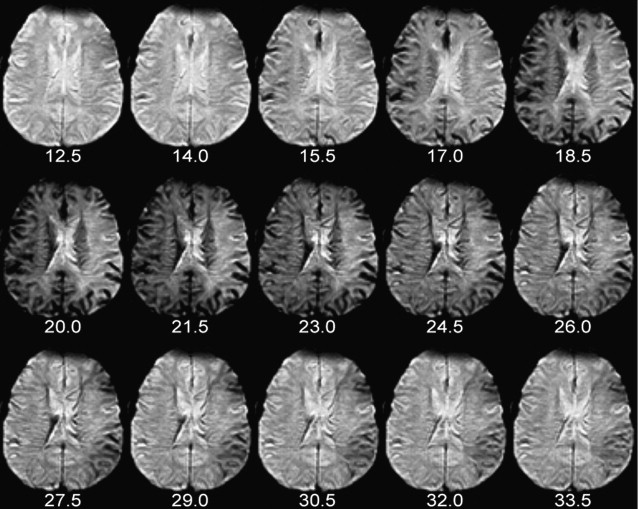
In DSC, susceptibility-sensitive images are acquired dynamically during the passage of a gadolinium-based contrast agent through the brain. As the contrast agent arrives in the brain and then washes out again, first the large arteries demonstrate a transient loss in signal intensity, followed by transient parenchymal signal loss as the contrast agent moves through smaller vessels, and then finally signal loss in the large intracranial veins ( Fig. 1 ). To create high-quality perfusion maps, the passage of contrast agent in each part of the brain must be measured with high temporal resolution. Ideally, images should be obtained no less frequently than one every 1.5 seconds for human stroke imaging, assuming a normal MTT of approximately 3 to 4 seconds. This is generally accomplished using an echo planar imaging (EPI) pulse sequence, which permits acquisition of an entire image slice with only a single radiofrequency excitation. Either spin-echo (SE) or gradient-echo (GRE) EPI images can be used. However, because SE EPI images are less sensitive to gadolinium’s susceptibility effects, using a SE EPI pulse sequence at 1.5 T requires injecting a larger dose of the contrast agent, typically 0.2 mmol/kg, while a standard dose of 0.1 mmol/kg is usually sufficient for GRE EPI imaging. However, because susceptibility effects are more pronounced at higher field strengths, the standard dose of 0.1 mmol/kg may be sufficient for SE EPI perfusion imaging at field strengths of 3 T or higher. Nevertheless, GRE imaging is performed more often than SE imaging at all field strengths. The pulse sequence parameters used at the authors’ institution are listed in Table 2 . All of the examples depicted in this review were generated using these parameters.
| Pulse sequence | Gradient echo, echo-planar |
| Orientation | Axial |
| Phase-encoding direction | Anterior-posterior |
| Repetition time/echo time/flip angle | 1500 ms/40 ms/60 degrees |
| Field of view | 22 cm |
| Matrix size | 128×128 |
| Slice thickness/interslice gap | 5 mm/1 mm |
| Number of slices | As many as permitted by scanner at TR = 1500 milliseconds (approximately 14) |
| Number of acquisitions | 80 |
| Pulse sequence duration: | 2 minutes |
| Contrast material | Gadopentatate dimeglumine, 20 mL, injected intravenously at 5 mL/s, beginning 10 seconds after initiation of the scan. Following the contrast agent injection, 20 mL of normal saline is injected at the same rate. |
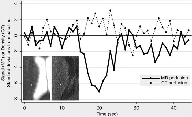
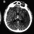
The physical basis of image contrast in DSC results in several noteworthy properties of the perfusion maps produced by DSC. First, DSC’s sensitivity to changes in precession frequency of all of the spins within each brain voxel gives the technique far greater sensitivity for detecting changes in contrast agent concentration than computed tomography (CT) perfusion imaging, which relies on the x-ray attenuation of an iodine-based contrast agent that remains within the intravascular space ( Fig. 2 ). CT perfusion postprocessing algorithms usually compensate for the far greater noise level within their source images by performing spatial and temporal blurring, which is not usually done in DSC postprocessing. Second, unlike CT perfusion imaging, which is equally sensitive to the presence of the contrast agent within vessels of all sizes, DSC produces different degrees of signal change for similar quantities of gadolinium in blood vessels of different sizes. GRE EPI is more sensitive to contrast agent in larger vessels, whereas SE EPI demonstrates greater sensitivity to contrast agent in smaller vessels. Some DSC pulse sequences exploit this vessel-size sensitivity by acquiring both SE and GRE images during the same contrast injection, enabling elementary measurements of the relative proportions of smaller and larger blood vessels. Although this interleaved technique has shown promise in assessing neovascularity within brain tumors, it is not generally used in acute stroke imaging. However, findings in animal models suggest that combining GRE-based and SE-based perfusion imaging may provide improved insight into tissue status after stroke.
Dynamic susceptibility contrast imaging: basic physics and image acquisition
Because currently available techniques quantify the passage of blood through vessels that are too small to visualize directly with standard clinical MR imaging scanners, MR perfusion imaging must rely on detection of tracer agents within blood, rather than direct visualization of the vessels. This review focuses on dynamic susceptibility contrast (DSC) imaging, the technique that is used for MR perfusion imaging of acute stroke in most clinical centers. Arterial spin labeling (ASL) is another technique for measuring perfusion without requiring exogenous contrast agents, which currently is rarely used in acute stroke imaging, because of its low signal-to-noise ratio, relatively long imaging times, and its difficulty in distinguishing between reduced blood flow and delayed transit times. Ongoing research seeks to eliminate artifacts, and ASL offers great potential for the future.
DSC uses a gadolinium chelate as an exogenous contrast agent. Although conventional contrast-enhanced MR imaging relies on the T1 effects of gadolinium to detect increased permeability of the blood-brain barrier, in DSC image contrast is based instead on gadolinium’s susceptibility effect, because the T1 relaxivity effect of gadolinium extends over extremely short distances. If the blood-brain barrier is intact, as is usually the case in acute stroke, only the approximately 1% to 7% of water spins that are also within blood vessels would experience an appreciable change in T1 relaxation, and the pulse sequence’s ability to detect small changes in local concentrations of gadolinium would be limited. However, the susceptibility effect of gadolinium ions inside of blood vessels extends over a range that is comparable in magnitude to the radius of the blood vessel, which is many orders of magnitude larger than gadolinium’s T1 effects. Therefore, all water spins within a voxel may be affected by the presence of the gadolinium, and the resulting signal change is much larger than the signal change that would have been caused by T1 effects.
In DSC, susceptibility-sensitive images are acquired dynamically during the passage of a gadolinium-based contrast agent through the brain. As the contrast agent arrives in the brain and then washes out again, first the large arteries demonstrate a transient loss in signal intensity, followed by transient parenchymal signal loss as the contrast agent moves through smaller vessels, and then finally signal loss in the large intracranial veins ( Fig. 1 ). To create high-quality perfusion maps, the passage of contrast agent in each part of the brain must be measured with high temporal resolution. Ideally, images should be obtained no less frequently than one every 1.5 seconds for human stroke imaging, assuming a normal MTT of approximately 3 to 4 seconds. This is generally accomplished using an echo planar imaging (EPI) pulse sequence, which permits acquisition of an entire image slice with only a single radiofrequency excitation. Either spin-echo (SE) or gradient-echo (GRE) EPI images can be used. However, because SE EPI images are less sensitive to gadolinium’s susceptibility effects, using a SE EPI pulse sequence at 1.5 T requires injecting a larger dose of the contrast agent, typically 0.2 mmol/kg, while a standard dose of 0.1 mmol/kg is usually sufficient for GRE EPI imaging. However, because susceptibility effects are more pronounced at higher field strengths, the standard dose of 0.1 mmol/kg may be sufficient for SE EPI perfusion imaging at field strengths of 3 T or higher. Nevertheless, GRE imaging is performed more often than SE imaging at all field strengths. The pulse sequence parameters used at the authors’ institution are listed in Table 2 . All of the examples depicted in this review were generated using these parameters.
| Pulse sequence | Gradient echo, echo-planar |
| Orientation | Axial |
| Phase-encoding direction | Anterior-posterior |
| Repetition time/echo time/flip angle | 1500 ms/40 ms/60 degrees |
| Field of view | 22 cm |
| Matrix size | 128×128 |
| Slice thickness/interslice gap | 5 mm/1 mm |
| Number of slices | As many as permitted by scanner at TR = 1500 milliseconds (approximately 14) |
| Number of acquisitions | 80 |
| Pulse sequence duration: | 2 minutes |
| Contrast material | Gadopentatate dimeglumine, 20 mL, injected intravenously at 5 mL/s, beginning 10 seconds after initiation of the scan. Following the contrast agent injection, 20 mL of normal saline is injected at the same rate. |
The physical basis of image contrast in DSC results in several noteworthy properties of the perfusion maps produced by DSC. First, DSC’s sensitivity to changes in precession frequency of all of the spins within each brain voxel gives the technique far greater sensitivity for detecting changes in contrast agent concentration than computed tomography (CT) perfusion imaging, which relies on the x-ray attenuation of an iodine-based contrast agent that remains within the intravascular space ( Fig. 2 ). CT perfusion postprocessing algorithms usually compensate for the far greater noise level within their source images by performing spatial and temporal blurring, which is not usually done in DSC postprocessing. Second, unlike CT perfusion imaging, which is equally sensitive to the presence of the contrast agent within vessels of all sizes, DSC produces different degrees of signal change for similar quantities of gadolinium in blood vessels of different sizes. GRE EPI is more sensitive to contrast agent in larger vessels, whereas SE EPI demonstrates greater sensitivity to contrast agent in smaller vessels. Some DSC pulse sequences exploit this vessel-size sensitivity by acquiring both SE and GRE images during the same contrast injection, enabling elementary measurements of the relative proportions of smaller and larger blood vessels. Although this interleaved technique has shown promise in assessing neovascularity within brain tumors, it is not generally used in acute stroke imaging. However, findings in animal models suggest that combining GRE-based and SE-based perfusion imaging may provide improved insight into tissue status after stroke.
Dynamic susceptibility contrast imaging: measurement of perfusion parameters
Overview
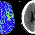
Direct inspection of DSC images can yield rudimentary information about regional brain perfusion, and this approach is sometimes useful when severe patient motion precludes additional postprocessing. However, under most circumstances, individual DSC images like those in Fig. 1 undergo additional postprocessing to produce maps of various perfusion-related parameters, in which each pixel’s value reflects a single scalar measurement that is derived from the signal intensity-versus-time function for the corresponding voxel. It is these maps that are interpreted in the clinical setting. Many different perfusion measurements can be derived from DSC images, but five are most commonly used: time to peak contrast concentration (TTP), CBV, CBF, MTT, and time at which the deconvolved residue function reaches its maximum value (Tmax).
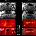
Examples of these five perfusion maps, illustrating each of the 4 abnormal perfusion conditions listed in Table 1 , are presented in Figs. 3–6 . As is evident from these examples, the various kinds of perfusion maps vary greatly in appearance, and they provide vastly different information about brain perfusion. Nevertheless, it has become commonplace for published stroke imaging articles to refer to these maps generically as “perfusion imaging,” and this has led to considerable confusion and inconsistency. Confusion surrounding the different types of perfusion maps is exacerbated by the fact that although most of these perfusion maps (specifically CBV, CBF, and MTT) ostensibly depict well-defined fundamental physiologic parameters, detailed examination of the algorithms that are used to compute them reveals several major technique-dependent artifacts. To best understand the use of perfusion imaging in the care of stroke patients, it is important to understand in some detail the postprocessing techniques that are used to create each kind of perfusion map, and the artifacts that they may introduce.
Time to Peak Concentration
Of the five parameters that are discussed here, TTP is the simplest to calculate and provides the least specific information about brain perfusion. In each voxel, TTP is the time at which signal intensity reaches its minimum, and therefore contrast concentration reaches its maximum. For example, for a particular DSC acquisition in which images are acquired every 1.5 seconds, possible TTP values could include 20.0 seconds, 21.5 seconds, 23.0 seconds, and so forth.
Numerous studies have used increases in regional TTP for putative identification of brain tissue that is threatened by ischemia, including one clinical trial that used diffusion-weighted imaging (DWI)-TTP mismatch to select patients for intravenous thrombolytic therapy outside of the usual 3-hour time window. The advantages of TTP in this role are that lesions in TTP maps are conspicuous and usually well defined, and that TTP is a reproducible technique, in that measurements obtained by different centers from a single data set are similar, with fewer technique-dependent artifacts to complicate interpretation. TTP is very sensitive to motion artifacts and noise, so some algorithms that perform motion correction and prefiltering will produce differing results. Some algorithms also perform curve fitting to obtain TTP. A primary disadvantage of using TTP is that TTP can be prolonged in a wide variety of acute and chronic hemodynamic conditions, in which tissue viability may or may not be threatened. As shown in Figs. 3–5 and Fig. 7 , TTP prolongation may be caused by reduced blood flow, but also occurs when the arrival of the injected contrast bolus is delayed, but CBF is normal. In some circumstances, TTP may even be prolonged in reperfused tissue whose CBF is higher than normal, tissue whose survival clearly is no longer threatened by ischemia.
Converting Signal Changes to Concentration Measurements
Calculation of all of the four remaining perfusion parameters that are discussed here relies on a common first step: conversion of each voxel’s signal intensity-versus-time curve into a contrast agent concentration-versus-time curve. To accomplish this conversion, the signal intensity-versus-time curve must be divided into two portions, reflecting signal intensity before and after arrival of the injected contrast bolus, respectively. Before bolus arrival, signal intensity fluctuates slightly, due to random noise, around a baseline value that is determined by time-invariant properties of the tissue within the voxel and the pulse sequence that is used. Preinjection points are typically averaged to produce an estimate of baseline signal intensity, S 0 . Following the arrival of the bolus, the concentration of gadolinium in a voxel can be derived from signal intensity by the equation
in which C ( t ) is the contrast agent concentration at a particular time t, S t is the signal intensity at that time, S 0 is the baseline signal intensity before the arrival of the contrast agent, and k is a constant whose value depends on the pulse sequence used, the manner in which the contrast is injected, and complex characteristics of the patient’s circulatory system that are difficult to model. Because the value of k is difficult to estimate, absolute perfusion measurements are difficult to obtain, and most perfusion maps provide only relative quantification of perfusion parameters. Although techniques have been proposed for computing absolute measurements of CBF with MR perfusion imaging, these measurements, like those obtained from CT perfusion imaging, typically vary by as much as a factor of 2 or 3, compared with those obtained by gold-standard methods such as xenon CT and PET.
Cerebral Blood Volume
Of the remaining four perfusion parameters (CBV, CBF, MTT, and Tmax), calculation of CBV is the simplest, requiring the fewest additional computational steps. Although CBV was one of the first perfusion parameters to be derived from MR perfusion imaging in human stroke, MR CBV maps historically have had little utility in acute stroke imaging, because the role that was presumptively assigned to them is better filled by DWI. The lesion seen on DWI is generally accepted to be the best available indicator of the irreversibly injured tissue in the infarct core. Several studies found that CBV maps often demonstrated a low-CBV lesion whose volume was small, like that of the DWI lesion, and that the volumes of both lesions served well as a lower limit of the volume of the infarct that was ultimately seen in later follow-up images. Because of these observations, it was suggested that CBV maps, like DWI, could be used to identify the infarct core. However, CBV maps were rarely used for this purpose in practice, because lesions in DWI images are far more conspicuous and clearly delineated than those in CBV maps. In addition, many of these studies used SE EPI for the data acquisition, which is more sensitive to smaller vessels that may manifest injury earlier than larger vessels, whereas currently the majority of clinical MR imaging centers use GRE EPI.
Interest in using CBV maps to define the infarct core increased greatly with the emergence of CT perfusion imaging. Although CT-based and MR-based techniques can provide similar perfusion maps, there is no CT equivalent for DWI, and so there is no accepted way to identify the infarct core without MR imaging. Some investigators have suggested that the core can be identified by CT-derived CBV maps, thereby obviating the need for DWI. This practice implicitly accepts that the significant proportion of core tissue that experiences spontaneous reperfusion will not be identifiable as such, and that the diagnosis of stroke may be missed if the entire infarct has reperfused. Even without reperfusion, the notion that CBV is reduced in the infarct core contradicts the physiologic principle that blood vessels dilate in underperfused tissue, in order to recruit additional blood flow. Although it has been hypothesized that CBV may drop when extremely low perfusion pressures cause vascular collapse, this phenomenon is poorly documented and its prevalence is unclear.
The apparent contradiction between MR-based and CT-based findings of reduced CBV in the infarct core, and theoretical and empirical predictions of elevated CBV, may be explained by artifactual flow-weighting and delay-weighting that are introduced by the algorithms used to calculate CBV. CBV theoretically can be calculated by integrating the area under the contrast agent concentration-versus-time curve, C ( t ), for the first pass of the injected contrast bolus through each voxel. However, measuring just the first pass is difficult, because recirculation usually results in the arrival of the second pass before the first pass is complete, and the two passes therefore are summed together in the measured C ( t ). Some researchers have attempted to extract the first pass of the contrast bolus by fitting gamma variates or other functions to the first portion of C ( t ). However, no particular model has been shown to reflect the first pass reliably.
Because of these challenges, CBV is usually calculated by numerically integrating the area under the entire C ( t ). This method produces truly accurate CBV measurements only for infinitely long scan durations because, as the time postinjection approaches infinity, contrast agent concentration in all parts of the brain approaches steady state. However, actual MR perfusion scans have finite durations, typically on the order of 60 seconds. During that time, the contrast agent concentration-versus-time curves in different parts of the brain may reflect different numbers of passes of the contrast agent. Specifically, in regions where the arrival of the contrast bolus is delayed, and/or low regional CBF results in a slower rate of arrival of the contrast bolus, C ( t ) is effectively truncated. Fewer passes of the contrast bolus will be recorded in a particular finite time period, and CBV will be underestimated, in comparison to other parts of the brain. In effect, CBV maps produced by this method are flow-weighted and delay-weighted.
Unfortunately, bolus arrival delay and decreased blood flow are common phenomena in acute stroke. When an injected contrast agent bolus reaches brain tissue via a pathologically narrowed artery, or via long collateral perfusion pathways, its arrival is delayed, and CBV is therefore underestimated. If the arterial lesion is severe enough to cause a CBF reduction, this too will cause underestimation of CBV. This artifact is mitigated by longer scan durations, and is exacerbated by shorter scan durations ( Fig. 8 ). Some centers have employed scans as short as 40 seconds, which usually is not long enough even to completely sample the first pass of the bolus in tissue with low CBF.
Related posts:
 Imaging Acute Stroke is Rapidly Evolving
 Arterial Spin Label Imaging of Acute Ischemic Stroke and Transient Ischemic Attack
 Intra-arterial Stroke Therapy: Recanalization Strategies, Patient Selection and Imaging
 Measuring Permeability in Acute Ischemic Stroke
 Noninvasive Carotid Artery Imaging with a Focus on the Vulnerable Plaque
 ASPECTS and Other Neuroimaging Scores in the Triage and Prediction of Outcome in Acute Stroke Patients
Stay updated, free articles. Join our Telegram channel

Full access? Get Clinical Tree


