This article provides an overview of relaxation times and their application to normal brain and brain and cord affected by multiple sclerosis. The goal is to provide readers with an intuitive understanding of what influences relaxation times, how relaxation times can be accurately measured, and how they provide specific information about the pathology of MS. The article summarizes significant results from relaxation time studies in the normal human brain and cord and from people who have multiple sclerosis. It also reports on studies that have compared relaxation time results with results from other MR techniques.
Overview
Relaxation is arguably the most important concept in MRI because it is the basis of and provides most of the contrast visible on conventional MRI, which plays a key role in the diagnosis and management of multiple sclerosis (MS). Many investigators have attempted to measure relaxation times in MS with the goal of obtaining more specific and accurate information about the disease. Although there has been significant progress in this area, relaxation time measurement is not yet a widely used tool for the investigation of MS pathology. Recent results suggest that relaxation time measurements can provide specific information about MS that cannot be obtained by other in vivo techniques.
This article provides an overview of relaxation times and their application to normal and MS brain and cord. The goal is to provide readers with an intuitive understanding of what influences relaxation times, how relaxation times can be accurately measured, and how they provide specific information about the pathology of MS. The article is organized into six sections. First, three relaxation times—T1, T2, and T2∗—are introduced, initially in the context of their behavior in simple water solutions and subsequently in central nervous system (CNS) tissue, where MR relaxation is much more complicated. The next section covers methods for accurate measurement and analysis of relaxation times in brain, highlighting the fact that CNS tissue is inhomogeneous and that this inhomogeneity can be planned for in the methodology. The article summarizes significant results from relaxation time studies in the normal human brain and cord and from people who have MS. Finally the article reports on studies that have compared relaxation time results with results from other MR techniques, including diffusion tensor imaging (DTI) and magnetization transfer imaging.
Although this article focuses primarily on T1, T2, and T2∗ relaxation times, susceptibility-weighted imaging (SWI), a T2∗ weighted technique is discussed. This article does not cover all relaxation time measurements (eg, T1ρ and T2ρ) because few MS studies have used these measurements.
T1, T2, and T2∗ relaxation times
Nuclear Magnetic Resonance
The phenomenon of nuclear magnetic resonance (NMR) enables us to obtain exquisite images from hydrogen nuclei in the brain. Hydrogen nuclei, or protons, from tissue behave like tiny magnets when placed in the magnetic field of an MRI scanner. In equilibrium, more protons are aligned parallel to the field than anti-parallel to the field, which results in a net magnetization vector along the magnetic field. If the net magnetization vector of the protons is tilted away from the MRI scanner field direction, it precesses about the direction of the magnetic field (like a top or gyroscope) at the resonance frequency, or Larmor frequency, ω o . ω o , which is determined by the Larmor equation, ω o = γB, where γ , the gyromagnetic ratio, depends on the nucleus and B is the magnetic field. For a 1.5-T magnet, the Larmor frequency for protons is 64 MHz. The magnetization vector is tilted out of equilibrium by applying external magnetic fields that oscillate at the Larmor frequency. The precessing magnetization produces a signal that can be picked up by a receiver coil and is used to create the MR image. The return of the net magnetization vector of the protons back to equilibrium is characterized by relaxation times T1, T2, and T2∗.
Relaxation Times
T1, the spin–lattice relaxation time (or longitudinal relaxation time), characterizes the return of the magnetization vector to align along the magnetic field direction. T2, the spin–spin relaxation time (or transverse relaxation time), describes the irreversible decay of the MR signal in the transverse plane, whereas T2∗ characterizes the actual measured decay of the MR signal. The T1 process involves an exchange of energy between the protons and the rest of the sample, or lattice, whereas T2 processes conserve energy. The next section provides a mechanistic description of T1 and T2 processes; readers who prefer a more intuitive picture of relaxation in tissue may skip to the following section.
T1 and T2 Processes
For a simple spin system consisting of a molecule with a single proton site, T1 and T2 are understood quantitatively in terms of fluctuating magnetic fields produced by adjacent protons undergoing molecular motions. Recall that protons behave like small magnets. When protons are located on molecules that reorient rapidly because of molecular tumbling and translational diffusion, they produce oscillating magnetic fields. Molecular motions, which are driven by the inherent kinetic energy of the molecules, are characterized by a correlation time, τ c , the time required for the molecule to undergo reorientation. The fluctuating magnetic fields caused by these molecular motions cause relaxation. The dependence of T1 and T2 on the correlation time of molecular motions and Larmor frequency is quantitatively expressed in equations 1 and 2 . The constant, K, is related to the strength of the interactions between adjacent protons.
1 T 2 = K ( 3 2 τ c + 5 / 2 τ c 1 + ( ω o τ c ) 2 + τ c 1 + ( 2 ω o τ c ) 2 )
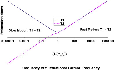
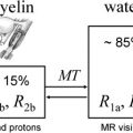
The simple model for relaxation described previously holds for simple spin systems such as water solutions but is unable to quantitatively characterize relaxation in brain that has multiple proton environments. Although the largest molecular component of brain is water (70%–80% by weight), the CNS is not a simple solution but rather consists of a complex arrangement of microscopic cellular structures. In brain, there are many different proton sites. Protons attached to macromolecules and lipids do not contribute directly to the signal we measure in MRI because their signal decays to zero in a few tens of seconds. The signal from protons attached to water in CNS tissue decays much more slowly and is fully accessible by MRI. Relaxation times for water in CNS tissue are strongly influenced by interactions between water and nonaqueous protons, however. In pure water, relaxation is well described by a simple process with a correlation time, τ c , of approximately 10 −12 seconds corresponding to the fast motion regime in which T1 = T2. In brain, water protons interact with other protons attached to molecules that move at a wide range of different frequencies (eg, low frequencies that arise from slow macromolecular reorientations to high frequencies that arise from fast small molecule tumbling). As a consequence, T2 times are shorter than T1 times in CNS tissue. T1 and T2 are also shortened in the presence of indigenous ions (eg, iron from hemoglobin or ferritin), which produce fluctuating magnetic fields at high frequencies.
Intuitive Picture of T1 and T2 in Brain
At 1.5 T, the T1 and T2 times for pure water are approximately 3 seconds, whereas the T1 time of water in brain is approximately 1 second and T2 times of water in brain are a few tens of milliseconds. This shortening in water relaxation times in CNS tissue is caused by interactions between brain water and nonaqueous tissue components, such as membranes and cytoplasmic proteins. Relaxation in brain is further complicated by the fact that local microscopic structures vary substantially within a typical imaging voxel volume of a few mm 3 . For example, glial cells have single plasma membranes, whereas myelinated neurons contain many membranes in close proximity. This microscopic heterogeneity results in substantially different relaxation behavior for water protons in different environments within a single voxel. As a further complication, boundaries between water environments in CNS tissue are blurred because of translational diffusion. Water molecules in pure water or dilute solutions undergo random motion, moving an average distance of R = (6Dτ) 1/2 in time τ, where D is the water diffusion coefficient. For a typical MR image obtained with an echo time (TE) of 60 milliseconds, free water in a solution moves over 30 μ. The barriers present in CNS tissue suppress water diffusion coefficients to less than one tenth that in free water, and water molecules move on average 5 μ in 60 milliseconds. Because of diffusion, parameters derived by MR are averaged over their values during the timescale of the measurement. Because T2 and T1 operate on different timescales (approximately 10 milliseconds to approximately 1 second), we observe different averages with these two parameters.
Manipulating T1 and T2 Times with Exogenous Contrast Agents
Exogenous contrast agents are used to investigate blood-brain barrier breakdown in MS. Gadolinium (Gd)-based contrast agents consist of Gd ions chelated by an organic molecule that protects the body from toxic effects of the free Gd ion. When the blood-brain barrier is sufficiently leaky, chelated Gd complexes can diffuse across the vascular wall, although animal studies present some evidence that there may be active transport of Gd. Water protons in the parenchyma are then exposed to intense fluctuating magnetic fields from the Gd ions. These additional high-frequency fluctuating fields cause a decrease in T1 and T2. This effect enables identification of regions of blood-brain barrier breakdown in MS brain that characterize enhancing lesions. By measuring changes in signal intensity in rapidly acquired brain images after injection of a bolus of Gd contrast into the venous system, it is possible to measure brain perfusion.
T2∗and Susceptibility-Weighted Imaging
Magnetic susceptibility is a concept that describes a substance’s ability to modify an applied magnetic field. The magnetic susceptibility, χ, is a constant that relates to the magnetization (M) of a substance by
with the external magnetic field H . This magnetization ( M ) shifts the actual magnetic field B from H as shown in equation 4 , where μ 0 = 4π 10 −7 VsA −1 m −1 denotes the permeability in a vacuum.
Depending on the sign of χ, materials are referred to as diamagnetic (χ < 0) or paramagnetic (χ > 0). Most tissues are diamagnetic (slightly repelled by a magnetic field). The main source of paramagnetism (form of magnetism that occurs only in the presence of an externally applied magnetic field) in the human body is iron. If a sample contains two or more compartments with different magnetic susceptibilities, static magnetic field inhomogeneities arise, which fall into two categories: (1) mesoscopic field inhomogeneities, which are field variations over distances longer than the water diffusion length during TE of an MR measurement but smaller than the voxel size, and (2) macroscopic field inhomogeneities, which vary over several voxels. In the human body, interfaces between air and tissue, bone and tissue, or veins and surrounding tissue are the main sources of field inhomogeneities. These inhomogeneities lead to an additional signal decay that is commonly characterized by a decay time of 1/T2′. The decay due to both T2 and T2′ relaxation is called T2∗ relaxation and obeys the simple equation
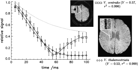
Equation 5 suggests that T2′ decay is exponential, but this is only true if the resonance frequency distribution caused by the static field inhomogeneities is Lorentzian (eg, for a large number of magnetic dipoles within a voxel). In general, T2′ is not monoexponential and not exponential at all. For a small number of dipoles, a vascular network, or macroscopic background field inhomogeneities the decay becomes nonexponential. In the presence of a single large blood vessel, the concept of an exponential decay also fails because the geometric relationship between field inhomogeneities and the voxel geometry (spatial resolution, slice orientation, imaging point spread function) plays an important role in signal formation. Venous vessels produce local field inhomogeneities, which depend on the venous blood oxygenation and the vessel’s orientation. For example, for a vessel parallel to the magnetic field, there are two discrete field strengths inside and outside of the vessel. Consequently, the spins inside and outside of the vessel have two discrete resonance frequencies that, when superimposed, lead to a distinct beat in the signal ( Fig. 2 ).
The blood oxygenation level dependency (BOLD) of the T2∗-weighted signal that is the basis of functional MRI and BOLD MR venography, currently called SWI, allows for the visualization of small venous vessels using deoxygenated venous blood as an intrinsic contrast agent.
T1, T2, and T2∗ relaxation times
Nuclear Magnetic Resonance
The phenomenon of nuclear magnetic resonance (NMR) enables us to obtain exquisite images from hydrogen nuclei in the brain. Hydrogen nuclei, or protons, from tissue behave like tiny magnets when placed in the magnetic field of an MRI scanner. In equilibrium, more protons are aligned parallel to the field than anti-parallel to the field, which results in a net magnetization vector along the magnetic field. If the net magnetization vector of the protons is tilted away from the MRI scanner field direction, it precesses about the direction of the magnetic field (like a top or gyroscope) at the resonance frequency, or Larmor frequency, ω o . ω o , which is determined by the Larmor equation, ω o = γB, where γ , the gyromagnetic ratio, depends on the nucleus and B is the magnetic field. For a 1.5-T magnet, the Larmor frequency for protons is 64 MHz. The magnetization vector is tilted out of equilibrium by applying external magnetic fields that oscillate at the Larmor frequency. The precessing magnetization produces a signal that can be picked up by a receiver coil and is used to create the MR image. The return of the net magnetization vector of the protons back to equilibrium is characterized by relaxation times T1, T2, and T2∗.
Relaxation Times
T1, the spin–lattice relaxation time (or longitudinal relaxation time), characterizes the return of the magnetization vector to align along the magnetic field direction. T2, the spin–spin relaxation time (or transverse relaxation time), describes the irreversible decay of the MR signal in the transverse plane, whereas T2∗ characterizes the actual measured decay of the MR signal. The T1 process involves an exchange of energy between the protons and the rest of the sample, or lattice, whereas T2 processes conserve energy. The next section provides a mechanistic description of T1 and T2 processes; readers who prefer a more intuitive picture of relaxation in tissue may skip to the following section.
T1 and T2 Processes
For a simple spin system consisting of a molecule with a single proton site, T1 and T2 are understood quantitatively in terms of fluctuating magnetic fields produced by adjacent protons undergoing molecular motions. Recall that protons behave like small magnets. When protons are located on molecules that reorient rapidly because of molecular tumbling and translational diffusion, they produce oscillating magnetic fields. Molecular motions, which are driven by the inherent kinetic energy of the molecules, are characterized by a correlation time, τ c , the time required for the molecule to undergo reorientation. The fluctuating magnetic fields caused by these molecular motions cause relaxation. The dependence of T1 and T2 on the correlation time of molecular motions and Larmor frequency is quantitatively expressed in equations 1 and 2 . The constant, K, is related to the strength of the interactions between adjacent protons.
1 T 1 = K ( τ c 1 + ( ω o τ c ) 2 + 4 τ c 1 + ( 2 ω o τ c ) 2 )
Related posts:

Stay updated, free articles. Join our Telegram channel

Full access? Get Clinical Tree


