Noise Reduction Methods

through the loop. Specifically, the flux can be expressed as the surface integral of the field ${\mathbf{B}}$ over the area of the pick-up loop: $\phi = \int {\mathbf{B}} \cdot {\mathbf{ds}}$ .

The first MEG measurements were performed with only one sensor (Cohen 1968, 1972). The number of sensors simultaneously detecting the flux at distinct locations was small until the 1980s when the size of the sensor array started to grow rapidly. Today, modern MEG systems contain hundreds of sensors (e.g. Clarke and Braginski 2006, Chap. 11). The multichannel output of these systems can be expressed as a time-varying vector in the signal space, a concept introduced in the 1980s (Ilmoniemi 1981; Ilmoniemi and Williamson 1987; Ilmoniemi et al. 1987). Sampling theory (Ahonen et al. 1993) is crucial for the design of sensor arrays as well as for understanding the physical aspects of the multichannel signals, especially their spatial complexity and information content.

Various system issues in multichannel MEG systems complicate the interference suppression and signal analysis (Clarke and Braginski 2006, Chap. 7). Sensors packed close to each other in a multichannel array always suffer from crosstalk phenomena to some extent. These couplings, of the order of 1 %, typically arise from inductive coupling between the pick-up coils and feedback currents of the neighbouring MEG channels. Such cross-talk between the channels distorts the signals even in the absence of any external interference or hardware calibration errors. Therefore, cross-talk should be computationally or experimentally determined and compensated for to get an estimate of the cross-talk-free signal. Alternatively, the signals could be compensated for cross-talk in the forward model. Another major concern possibly violating our assumption of the direct applicability of Maxwell’s equations on measured signals are the calibration errors. For example, the electronic components used to transform the actual magnetic flux to a voltage may contain gain errors distorting the measurement. Manufacturing of the sensors is not infinitely accurate; there may be slight variations in the surface areas of the pick-up loops, locations and orientations of the sensor may deviate from the nominal ones, and the gradiometers may exhibit small imbalances. Therefore, it is important to calibrate the system as accurately as possible before estimating any source parameters from the data with mathematical models.

In this chapter, we concentrate on interference suppression methods operating at the sensor level of a multichannel MEG system. We do not assume any specific neural source model although some source modeling approaches, such as the beamformer, may also efficiently suppress interfering signals. We will mainly describe approaches for processing of the sensor-level data that can subsequently be used for analysis with any desired source modeling method. Regarding nomenclature, although “noise” is a commonly used general term to describe all kinds of magnetic disturbance fields and artifacts, we prefer to classify different types of MEG disturbance as follows: our use of “interference” will refer to non-physiological sources that are clearly unrelated to the MEG sensor array whereas our use of “noise” will refer to sensor or radiation-shield noise caused by random processes.

1.2 Sampling of the Neuromagnetic Field

All interference suppression methods make assumptions about the separability and detectability of interference and signals of interest. Such assumptions may include a priori information about the spatial, temporal, or spectral features characteristic to the different signal components. One of the fundamental questions is whether we can decompose the multichannel measurements into unique subsets of basic components, some containing only interference and others only neural signals.

In the spatial domain, the number of degrees of freedom, or the effective rank of the neuromagnetic data, has been extensively studied in the past (Ahonen et al. 1993). This spatial sampling theory for MEG is based on the fact that a multichannel MEG measurement can be considered as spatial sampling of the continuous neuromagnetic field. The theory shows that the measurable MEG signals are limited to the low end of the spatial-frequency spectrum. As a practical consequence, there is an upper limit to the number of sensors and a lower limit to the minimum distance between adjacent sensors. Specifically, it has been shown that for MEG signals measured at the minimum distance

, the contribution of spatial frequencies higher than

is below the sensor noise and therefore insignificant. Thus, the part containing biomagnetic information in the measured signals is limited in spatial complexity, which also means that the number of degrees of freedom of MEG data is limited. Although this reduces the effective rank of the data to about 100, hundreds of MEG channels are needed to reliably estimate the basis components spanning all detectable signals (e.g. Nenonen et al. 2004; Taulu and Kajola 2005).

1.3 Challenges Specific to MEG

The basic challenge of MEG stems from the fact that the neural currents are weak and aligned coherently in the brain only over a short distance, and the associated magnetic field is measured by sensors outside of the head. Additionally, with SQUID-based detectors, the sensor-to-source distance is further increased by the necessary thermal insulation layer of the helium dewar, about 20 mm. Consequently, the amplitude of the neuromagnetic signal detected in MEG is in the range from 10 to 1,000 fT.

The weakness of the signal can be overcome by increasing the sensitivity of the sensors; however, sensors that are more sensitive are also more susceptible to ambient interference fields, which may eventually exceed the dynamic range of the sensors. Clinical environments are often magnetically noisy, with a variety of electrical equipment radiating magnetic interference not only at the power line frequency and its harmonics, but also across a wide frequency range reaching from near DC up to several GHz. Interference at the lower end of the frequency range is usually due to traffic (cars, trains, trams) and large moving objects inside the building (e.g. elevators). The typical low-frequency peak-to-peak variation of the magnetic field in such an environment is a couple of $\mu{\rm T}$ .

To measure 10-fT signals of interest on top of 1- $\mu{\rm T}$ interference, one would need a sensor with a dynamic range exceeding 8 orders of magnitude. To date, no magnetic sensor exists with a linear response over such a wide dynamic range. The linearity of the sensors, on the other hand, is a necessary prerequisite for successful signal processing and source analysis. Therefore, an efficient means to reduce the actual physical magnetic interference is necessary for feasible MEG recordings and analysis, especially in a clinical environment. When hardware-based magnetic shielding is sufficient to keep the sensors within their linear operating range, the remaining interference can be further reduced by multichannel signal processing methods, such as spatial and temporal filtering.

Another challenge specific to MEG is the possible movement of the subject’s head during recording. The physical sensor array of the MEG system is stationary. Movement-related distortion of the signal biases source localization and is more challenging with MEG than with the EEG method where the electrodes are attached on the scalp and do not move with respect to brain. To fully benefit from the MEG method’s better source localization capability, one must ensure that the accurate location of the head relative to the sensor array is known at all times during the MEG recording.

1.4 Sources of Interference and Noise

The largest-amplitude ambient magnetic fields usually arise from traffic outside of the building. Elevators and MRI magnets operated close to MEG, and even doors made of magnetic material are potential sources of magnetic interference inside of the building. In urban environments, cars on nearby streets, trains and metros cause low-frequency peak-to-peak variations of magnetic field which are typically in the range 1–3 $\mu{\rm T}$ .

When a vehicle moves at a distance of

with velocity

, the frequency range of the resulting interference is around

. For example, cars driving at 50 km/h at a distance of 30 m or a train passing by at 200 km/h at a distance of 100 m result in low-frequency field variations at around 0.5 Hz.

In this frequency range the shielding factor of a typical magnetically shielded room (MSR) is rather low, about 100 (40 dB). Therefore, operating magnetometer sensors in an MSR with 1- $\mu{\rm T}$ ambient interference from traffic requires sensors with higher than 10-nT dynamic range, if no other means of interference rejection is used.

Because the shielding factor of an MSR rises steeply with increasing frequency, the low-frequency interference present in the environment will typically dictate the required hardware shielding performance at a specific MEG site. For example, interference at powerline frequencies 50/60 Hz seldom exceeds 1 $\mu{\rm T}$ in clinical environments, and is thus sufficiently dampened by a typical MSR which easily attains a shielding factor in the range of $10^{5}$ (100 dB) at these frequencies. An example of low- and line-frequency interference inside a magnetically shielded room is shown in Fig. 1.

Fig. 1

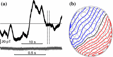
a An example of a single magnetometer (over the occipital region) signal recorded without a subject in the magnetically shielded room. The inset shows a 1-s epoch of the data which reveals the line-frequency contamination. b Spatial distribution at the time of the largest amplitude of the signal shows a homogeneous field distribution. The view is from the top of the sensor array, and the circles indicate the locations of the 102 magnetometers of the Elekta Neuromag MEG system. Blue and red lines indicate magnetic field flux into and out of the array surface, respectively. The step between adjacent contour lines is 20 pT

At radio frequencies up to several GHz, an MSR should maintain a shielding factor of about $10^{5}$ or higher. Although these frequencies are much higher than any brain signals and thus irrelevant for MEG, the shielding is still required because the functioning of DC SQUIDs involves intrinsic frequencies in the GHz range, related to the superconducting tunnel junctions whose so-called Josephson frequency is at 4.8 GHz for a bias voltage of 10 $\mu{\rm V}$ (see, e.g., Clarke and Braginski 2006). Modern digital equipment may cause strong electromagnetic radiation in this frequency range, and would severely disturb unshielded SQUID-based sensors.

The sources of interference and noise mentioned above are related to the installation site of the MEG device. In addition, there are numerous interference sources that are related to the MEG technology itself. Some of them cannot be compensated for by the MSR because they stem from the MSR itself or from sources inside of the MSR. For example, the walls of the MSR are made of conductive and magnetic material, which may result in magnetic interference by two mechanisms. The thermal currents in the walls of a typical MSR generate a magnetic field noise density of about 2 fT/ $\sqrt {\text{Hz}}$ (Nenonen et al. 1996). Also, small vibrations of the walls result in magnetic interference typically seen as 10–30-pT peaks in the frequency band 13–30 Hz. These peaks result from the high-Q-value eigenmodes of the MSR walls and ceiling that are driven by the vibration of the building and the infrasound due to forced ventilation.

Another vibration-related artifact in MEG signals arises from the mechanical movement of the MEG device itself in the remanence field inside of the MSR. The maximal amplitude of this type of artifact in magnetometer sensors can be estimated by multiplying the remanence field by the vibration-related rotation angle. The remanence field in a typical MSR is 100 nT. Assuming the vibrational rotation to be a 10- $\mu{\rm m}$ movement of the sensor helmet around an axis one meter away from the helmet, we observe 1 pT magnetic signal due to this vibration.

All metal, magnetic or conductive, components of the MEG device are potential sources of magnetic interference. Most of these sources can be eliminated by proper design of the equipment. After careful design, the dominant device-related source of magnetic interference is typically the thermal insulation (super insulation) covering the sensor area of the dewar, which is necessary to keep the liquid helium boil-off rate below 10 l per day. In modern MEG devices this noise contribution is below 3 fT/ $\sqrt {\text{Hz}}$ . Any auxiliary devices such as stimulators, cameras, speakers or microphones used inside of the MSR are also potential sources of severe interference. The compatibility of these devices with the MEG method must be carefully verified case by case.

Finally, the recorded MEG signals contain sensor noise related to the SQUIDs and their readout electronics. The pick-up antennas in a modern MEG device, having about 300 sensors in total, are relatively small. Therefore, to achieve adequate field sensitivity, it is necessary to minimize the electronics-related noise contribution. This can be done, for example, by applying pre-amplifier noise cancellation based on positive feedback (Kiviranta and Seppä 1995). In this way, the noise in individual MEG channels can be kept at the level of 3–4 fT/ $\sqrt {\text{Hz}}$ in the white noise range and at about (6/f) fT/ $\sqrt {\text{Hz}}$ at low frequencies (1/f-noise). There are also other device-related non-idealities that manifest as distortion and bias in the recorded data. Such factors include, for example, errors in calibration, location, and orientation of individual sensors, as well as imbalance of gradiometers and cross-talk between the channels. Most of these non-idealities, often seen as a kind of “DC-interference”, can be well characterized and compensated for by modern software methods that are discussed in detail in Sect. 3.

In addition to the ambient and device-related noise and interference mechanisms described above, the subject studied—or patient in case of clinical MEG—may also be a source of severe interference. This applies especially in clinical work where patients may often have dental braces, therapeutic stimulators, or magnetic residue from prior surgical operations on or inside the skull. Prior to the invention of advanced software-based methods for interference rejection, such magnetic components in the body were considered a contraindication for a meaningful MEG study. The software methods to suppress disturbances caused by magnetism in patients are discussed in detail in Sect. 3.

2 Conventional Interference Reduction Methods

2.1 Magnetic Shielding

As mentioned in the previous section, the basic method of interference reduction that has been in use since the very beginning of neuromagnetic studies (Cohen 1970) is to use a magnetically shielded room (MSR). Figure 2 illustrates the principle of magnetic shielding and shows a commercial three-layer room. MSR is a room-size metal enclosure constructed using layers of both highly conductive metal, usually aluminum or copper, and metal with high permeability (see e.g. Kelhä et al. 1982). Mu-metal is a commercial name for a variety of nickel-iron alloys having a dynamic (initial) relative permeability as high as 50,000.

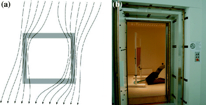
Fig. 2

a Principle of magnetic shielding. Layers of aluminum and mu-metal provide a path for magnetic field lines around the enclosure. b A three-layer magnetically shielded room (Imedco AG, Hägendorf, Switzerland) at the O.V. Lounasmaa Laboratory of Aalto University (Espoo, Finland)

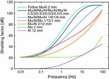
The shielding performance of a MSR is usually described by a frequency-dependent shielding factor which is the ratio between the external interference field $B_{\text{ext}} (f)$ and the corresponding value of field inside of the shield $B_{\text{in}} (f)$ , that is, $S(f) = B_{\text{ext}} (f)/B_{\text{in}} (f)$ . The shielding effect of a metallic magnetic shield made of conducting and high-permeability material is based on two mechanisms: polarization of the high-permeability metal, and eddy currents induced by varying magnetic field. These mechanisms are demonstrated in Fig. 3 where the shielding performances of different wall compositions, with equal proportions of mu-metal and aluminum, are compared.

Fig. 3

Optimization of aluminum/mumetal-based MSR wall structure. Estimated shielding factors of four different Al/mu-sandwich structures are shown. The scattering matrix model for concentric spherical shells (e.g., Kelhä et al. 1982) with inside radius 1.9 m is used in the calculation. The layers in the 2-, 3-, 4-, and 8-layer sandwiches are in surface-to-surface contact, and the amount of metal is kept constant in all four structures; 2 mm of mu-metal and 12 mm of aluminum in total. For the electrical conductivity of aluminum and mu-metal, and for the relative permeability of mu-metal we have used $3.57 \times 10^{7} (\Omega {\text{m}})^{ - 1}$ , $1.82 \times 10^{6} (\Omega {\text{m}})^{ - 1}$ , and 16,000, respectively. For reference, the $$S(f)$$

-curves of 12 mm of mere aluminum, and 2 mm of mere mu-metal are shown by the two lowermost curves. For mere aluminum, the shielding is negligible below 0.1 Hz, and above that grows proportional to $$f$$

due to induced global eddy currents. The skin depth of aluminum is so long that no skin effect, that is, exponential growth of $$S(f)$$

, is evident even at 100 Hz. This is because of the low relative permeability of aluminum. The second lowest curve is for 2-mm mu-metal showing a 20-dB shielding down to DC but no global current shielding regime, because of low electrical conductivity of mu-metal. Instead, a skin effect regime with exponential growth of $$S(f)$$

is starting to show up above 10 Hz. Keeping the total amount of metal constant, but increasing the number of layers in the al/mu-sandwich reduces the skin depth and the frequency at which the skin effect sets in. With an increasing number of layers in the sandwich, the shielding factor at a given frequency between 0.5 and 100 Hz increases and the $$S(f)$$

-curves asymptotically approach the uppermost curve showing the shielding obtained with an “infinite number” of layers, that is, a 2-mm thick shell made of fictive “Al/mu-alloy” having the electrical conductivity of a 12-mm thick aluminum plate, and the relative permeability of mu-metal. The saturation of $$S(f)$$

at 115 dB is due to the openings in the MSR wall

At frequencies below 0.1 Hz, where induction is negligible, the polarization of the high-permeability material is the only mechanism providing magnetic shielding. When the frequency increases, the induction mechanism starts to have an effect on the shielding. In this frequency range, additional shielding is provided by the “global” eddy currents induced to run in the conducting walls around the entire room. This additional shielding effect sets in at the frequency determined by the resistance of the conductive wall and the inductance related to these “global” currents. The related shielding effect grows proportional to the frequency, as shown by the lowermost $$S(f)$$

-curve in Fig. 3. When the frequency is further increased, the induced currents on the outer surface of the wall start to shield the inner parts of the wall, and the shielding starts to grow exponentially with increasing frequency. This is the well-known skin effect, with a skin depth given by $\delta = 1/\sqrt {\pi f\mu \sigma }$ . Here $\sigma$ and $\mu$ are the conductivity and permeability of the wall.

Since the construction of the first room-size magnetic shield in 1962 (Patton and Fitch 1962), a variety of different multilayer MSRs have been manufactured for biomagnetic purposes. To obtain increasingly better magnetic shielding performance, the amount of metal and the number of metal layers has been increased up to the record number of eight (Bork et al. 2001). Such a huge MSR with 6 × 6 × 6 m³ external dimensions and a total of 24.3 tons of mu-metal provides excellent magnetic shielding even at very low frequencies. While this type of shielding is extremely useful in scientific research requiring magnetically disturbance free environments, it is not practical for clinical MEG use.

As a solution for the need of compact and lightweight MSRs for clinical MEG applications, designs with a total MSR weight below 5 tons and external dimensions of 3 × 4 × 2.5 m³ have been developed during the past ten years (for performance evaluations, see Parkkonen et al. (2006) and de Tiège et al. (2008)). To ensure sufficient shielding performance of these light MSRs with reduced amount of mu-metal, special attention has been paid to the joints between the metal wall elements to guarantee optimal electric and magnetic conductance across the joints (Simola et al. 2005). Also, several conductive aluminum layers and high-permeability mu-metal layers have been interleaved to reduce the effective skin depth of the wall structure (Simola 2003). This lowers the frequency at which the skin effect and the related exponential growth of the shielding factor $$S(f)$$

with increasing frequency sets in, thus increasing the shielding performance at frequencies above 0.5 Hz; see Fig. 3.

To support the magnetic shielding provided by a MSR, several active shielding concepts have been proposed and realized. The simplest method to actively counteract ambient magnetic interference consists of a magnetic sensor—a three-axis fluxgate, for example—located in the vicinity of the MSR, and three orthogonal sets of coils wound on the outside of the MSR. The fluxgate records the variations of the ambient field and controls a current supply that feeds the coil sets to produce a field that counteracts the ambient field variations at the location of the MSR. This method is called feedforward active compensation. In this arrangement the fluxgate has to be located far from any local sources within the building, and at a sufficient distance from the compensation coils. The feedforward system works well against distant interference sources that produce a nearly uniform field. With this method a typical achievable shielding factor against such interference is in the range 10–50 (20–35 dB).

If the fluxgate is moved closer to or within the coil system, the arrangement turns into a feedback system that keeps the magnetic field constant at the location of the fluxgate, providing an alternative approach to construct an active compensation system. The fluxgate cannot be located inside the MSR because the inductive time constant of the MSR leads to a relatively long time delay between $B_{\rm ext} (t)$ and $B_{\rm in} (t)$ , typically 2–3 s. A novel feedback active compensation method based on the MEG sensors and compensation coils inside the MSR will be described below in Sect. 3.5.5.

2.2 Gradiometrization

Another hardware-related interference rejection method, which has been utilized since the early days of biomagnetism, is the use of gradiometers instead of simple magnetometers. Zimmerman and Frederick (1971) used an axial gradiometer consisting of two oppositely wound co-axial coils, while Cohen (1979) utilized a planar gradiometer where the coils are on the same plane (see Fig. 4).

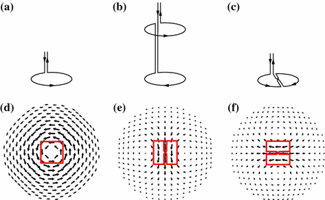
Fig. 4

Some pick-up coil geometries: a magnetometer, b co-axial first-order gradiometer, and c planar first-order gradiometer. The leadfield, or sensitivity, patterns of d magnetometer and axial gradiometer measuring $B_{z}$ , e planar gradiometer measuring $dB_{z} /dx$ , and f planar gradiometer measuring $dB_{z} /dy$

A first-order gradiometer has a pick-up antenna consisting of two loops that are planar, parallel, and usually identical in size and shape. The loops are oppositely wound and located in space so that one loop is translated from the other by a vector ${\mathbf{h}}$ . The length $$h$$

is called the baseline of the gradiometer. If ${\mathbf{h}}$ is parallel to the common normal ${\mathbf{n}}$ of the loops, the gradiometer is called axial. In the case of a planar gradiometer, ${\mathbf{h}}$ is orthogonal to ${\mathbf{n}}$ . In principle, ${\mathbf{h}}$ and ${\mathbf{n}}$ could be at any angle relative to each other but axial and planar are the two gradiometer types most commonly used.

The signal of a gradiometer MEG channel is proportional to the net magnetic flux through the pick-up antenna. If the field contains gradients up to second order only and the gradiometer is ideal this flux is given by

$g = A{\mathbf{n}}^{T} \left( {\begin{array}{*{20}c} {\partial B_{x} /\partial x} & {\partial B_{x} /\partial y} & {\partial B_{x} /\partial z} \\ {\partial B_{y} /\partial x} & {\partial B_{y} /\partial y} & {\partial B_{y} /\partial z} \\ {\partial B_{z} /\partial x} & {\partial B_{z} /\partial y} & {\partial B_{z} /\partial z} \\ \end{array} } \right){\mathbf{h}}$

(1)

where A is the area of one gradiometer loop.

For geometrical reasons, gradiometer antennas composed of identical oppositely-wound loops are totally insensitive to a uniform field of any direction. Consequently, they rather effectively reject interference from any sources far away from the MEG device. In practice, the interference rejection ratio of gradiometers is limited by the fact that a typical interference field is not exactly uniform, and that the geometry of the gradiometer is not ideal. The geometric non-ideality of a gradiometer is called imbalance. The signals from near-by sources, the brain signals, are highly non-uniform and therefore attenuated only slightly. Typically, for a gradiometer in a MSR, the signal-to-interference ratio for ambient interference is approximately by a factor of 100 higher than for simple magnetometers.

The interference signal in ideal gradiometers, related to relatively smooth interference fields, is well described by Eq. (1). When dealing with the signals of interest in MEG, which are related to neural current distributions, the signal in a MEG channel is better described by using the concept of a lead field ${\mathbf{L}}({\mathbf{r}})$ , defined by the expression

$b_{k} = \int_{{v^{'} }} {\mathbf{L}}_{k} ({\mathbf{r}}') \cdot {\mathbf{J}}({\mathbf{r}}')dv^{\prime}$

(2)

where the output of channel $$k$$

, $b_{k}$ , is obtained as the projection of the current distribution ${\mathbf{J}}({\mathbf{r}}')$ on the lead field, or sensitivity pattern, ${\mathbf{L}}_{k} ({\mathbf{r}}')$ .

The two types of gradiometers, axial and planar, have different sensitivity patterns (Fig. 4). An axial gradiometer has a similar lead field as a magnetometer: zero for sources directly under the sensor, otherwise wide circular pattern with the maximum sensitivity some distance sideways. Thus, a single axial gradiometer can detect neuromagnetic signals from a wide region in the brain, but is also sensitive to interference caused by sources near to the sensor. Planar gradiometers in turn have very compact lead fields, which exhibit the maximum directly under the sensor.

2.3 From Single-Channel to Multichannel MEG

In the early days of biomagnetism, MEG devices were comprised of one sensor channel only. Any feature in the signal could be from the brain, environment, or electronics. Instrumentation developed during the years, and the number and size of the sensor arrays increased gradually. Figure 5 illustrates the evolution of multichannel MEG sensor array from a small-size four-channel axial gradiometer to 306-channel whole-head system combining magnetometers and planar gradiometers. Modern whole-head MEG arrays have facilitated development of effective multichannel signal processing and analysis methods, which are discussed in Sect. 3. Design of multichannel sensor arrays involves several parameters, such as the number of channels, geometry of the pick-up coils, internal noise level of the sensors and so on. Detailed comparisons of the advantages and disadvantages of the arrays of axial and planar sensor types have been presented in the literature (Ahonen et al. 1993; Vrba and Robinson 2002; Nenonen et al. 2004).

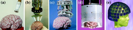
Fig. 5

Evolution of MEG devices: a 4-channel axial gradiometer system, b 7-channel axial gradiometer system, c 24-channel planar gradiometer array, d 122-channel planar gradiometer helmet, e 306-channel whole-head system combining 102 magnetometers and 204 planar gradiometers. (a–d: Courtesy of Dr Jukka Knuutila, Elekta Oy; e: Courtesy of Dr Mika Seppä, O.V. Lounasmaa Laboratory, Aalto University)

2.4 Reference Sensors

A method distantly related to the gradiometer concept is the use of reference sensors, which consists of an array of extra magnetic sensors located typically 20 cm above the MEG sensor helmet. The idea is that the reference sensors are so far from the source of interesting signals that they only detect interference. This measured interference can be modeled, either by a physical model or statistically, and then subtracted with proper weighting coefficients from the signals of the MEG channels. Because of the required extra hardware and the modeling and subtraction, the reference sensor method can be considered a combined hardware/software method.

In the reference-sensor method the interference contribution at the primary MEG sensors is extrapolated from the signals in the reference sensors by expanding the magnetic field into a Taylor series about the origin at the primary sensor. Synthetic first-, second- and third-order gradiometers can be formed in this manner (Vrba and Robinson 2001). Magnetometers and gradiometers can serve both as primary and as reference sensors. Synthetic third-order gradiometers reduce the environmental interference substantially. In order to avoid increasing the sensor noise, the reference sensors should have a higher gain than the primary sensors. Synthetic gradiometers have been demonstrated to operate even without a magnetically shielded room in an environment with low magnetic interference level.

2.5 Limitations

All the traditional interference rejection methods described above are in use at many MEG sites and have proven to work and to be sufficient in most cases to enable proper functioning of the MEG device. The main problem with the passive shielding method is the large size, heavy weight and high price of the MSR. Also, the need to isolate the patient behind a closed door may hamper clinical work. Lighter passive magnetic shields would boost the clinical use of MEG.

A relatively simple way to assist passive shielding is to use feedforward active compensation. The basic problem with this method of active compensation is related to the local sources in the vicinity of the MSR and the fluxgate sensor. If there are many such sources, it is impossible to set the system up properly and the arrangement may even amplify the interference from sources close to the fluxgate.

The basic shortcoming of the reference sensor method is related to the fact that the interference inside of the MSR may still be 1,000 times higher than the brain signals. Therefore, to be able to properly subtract the interference, one should know it at the location of each sensor with an accuracy better than one per mille (0.001). This is not possible when the interference needs to be extrapolated from the signals of only 10–30 reference sensors located at a 20-cm distance from the primary MEG sensors.

The conclusion is that improved interference rejection methods are needed, specifically to develop MEG towards clinical use. For clinical installations, it is not always possible to select the magnetically most silent location in the hospital. Also, clinical patients cannot be chosen for subjects as freely as in basic neuroscientific research. Patients may also have therapeutic stimulators that are magnetic or there may be magnetic residue from previous surgery in their body. In addition, patients and healthy volunteers often show interference from biological sources such as the eyes and cardiac muscle; see Parkkonen and Salmelin (2010) for typical examples. None of the methods described above are useful against such interference.

3 Modern Approaches to Noise Reduction

3.1 Mathematical Representation of Multichannel MEG Signals

We will concentrate on mathematical noise reduction methods and start from the basic principles of computational signal representation. These basic concepts are a necessary prerequisite for the understanding of novel algorithms used in MEG today.

As explained above, a common way to express the signals of individual MEG channels is the leadfield representation of Eq. (2), which shows how the output of channel $$k$$

, $b_{k}$ , is obtained from the current distribution ${\mathbf{J}}({\mathbf{r}}')$ as the projection of the current distribution to the lead field, or sensitivity pattern, ${\mathbf{L}}_{k} ({\mathbf{r}}')$ . MEG sensors are sensitive to both neural currents and currents related to interference but usually the lead fields are computed for neural currents only with the assumption that the measured data are sufficiently clean. Figure 4 shows examples of lead fields of magnetometer and gradiometer channels. The wide-spread sensitivity pattern of the magnetometer indicates that the magnetometer picks up signal from a large portion of the source volume, including deep structures in the brain. Similarly, magnetometers are also quite sensitive to external interference signals, which are spatially relatively uniform. On the other hand, the gradiometer channels are very focal and most sensitive to the superficial parts of the brain and insensitive to homogeneous interference fields.

Modern MEG devices contain hundreds of channels and the whole sensor array discretizes the continuous field distribution into a signal vector $s(t) = [s_{1} (t)\,s_{2} (t) \ldots s_{N} (t)]$ at any given time $$t$$

. This

-dimensional vector representation allows us to utilize linear algebra in the signal processing of MEG. From now on, we will call the set of measurable signal vectors the signal space of MEG and show that different subspaces can be distinguished in the signal space. The concept of signal space was first introduced in MEG already in the 1980s (Ilmoniemi 1981; Ilmoniemi and Williamson 1987; Ilmoniemi et al. 1987) and it has thereafter been the basis of several efficient signal processing algorithms.

3.2 Common Distortion Mechanisms of MEG Signals

The basis of any model applied to a multichannel MEG recording is the assumption that the sensors can be considered independent. For example, according to this assumption, a particular forward model can be computed by evaluating the magnetic flux at individual sensors merely based on the geometry of the associated source model and the sensor itself without considering the signals of other sensors. In reality, however, sensors always have some degree of coupling between each other. Therefore, instead of measuring the pure magnetic flux $\phi_{i}$ , channel $$i$$

detects the distorted signal $\phi_{i}^{'}$ due to the coupling of all other channels through the so-called cross-talk coefficients $k_{ij}$ , i.e.,

$\phi_{i}^{'} = \phi_{i} + \sum\limits_{j = 1}^{N} k_{ij} \phi_{j}^{'} ,$

(3)

where $k_{ii} = 0.$ Cross-talk arises e.g. from mutual inductance between sensors or electronics-based couplings. An efficient way to reduce cross-talk is to keep the current of the pick-up coils at zero by feedback, which eliminates the inductive coupling between the pick-up coils. Some cross-talk, however, always exists and it is important to estimate the coefficients $k_{ij}$ either computationally or to measure them directly by sequentially feeding a current to each sensor and detecting the response of other channels to this test current (Taulu 2000). Computational means include a model for the mutual inductance between sensors, which can be based, e.g., on analytical formulae between wire elements of the flux transformers. Once the coefficients $k_{ij}$ have been determined, the above equation can be written in the matrix form

$\phi^{'} = \phi + K\phi^{'}$

(4)

from which the cross-talk-corrected estimate can be computed as

$\phi = \left( {I - K} \right)\phi^{'} .$

(5)

In addition to the cross-talk, hardware-originating signal distortion arises due to errors in the calibration coefficients and geometrical imprecision, such as position and orientation errors of the sensors, and imbalance of gradiometers. If the expected field-to-voltage calibration coefficient of channel $$i$$