, which can be assumed to be two dimensional without a loss of generality, and impulse response  . Let
. Let  be squared area of the size
  , and let
  be a continuous function of fast decay whose Fourier transform
  is supported inside the circle
  , i.e.,
  if
if  of the imaging system is modeled as a convolution

(8.1)
 is the input signal. It is supposed that
  is integrable on
  . Then
  can be represented by the Fourier series
(8.2)
 and
and
(8.3)
Since the impulse response  is band limited with the bandwidth
  , the series (8.2) can be truncated:
with

and

is band limited with the bandwidth , the series (8.2) can be truncated:(8.4)
(8.5)
(8.6)
That is, the output  is a trigonometric polynomial and, consequently, can be uniquely recovered from its samples (see, e.g., [1]) measured over the rectangular grid
  Hence, under certain idealizing assumptions, the continuous image can be identified with its samples.
is a trigonometric polynomial and, consequently, can be uniquely recovered from its samples (see, e.g., [1]) measured over the rectangular grid Hence, under certain idealizing assumptions, the continuous image can be identified with its samples.We refer to the matrix  as a digital image of the input signal
  . In the following, we call the number
  the resolution limit of the imaging system, meaning that
  is the maximal resolution that can be achieved with this system. Clearly, for the case considered here, the value
  coincides with the Nyquist frequency of the imaging system.1
as a digital image of the input signal . In the following, we call the number the resolution limit of the imaging system, meaning that is the maximal resolution that can be achieved with this system. Clearly, for the case considered here, the value coincides with the Nyquist frequency of the imaging system.1 Finally, we point out that extending the matrix  periodically with the period
  ,
,  , we can write
which is the standard notation for the discrete 2D Fourier transform.
periodically with the period , , we can write(8.7)
8.2 Image Processing
In practice, we do not have to deal with the image  but with its corrupted version

where  is the random value referred to as system noise. For an X-ray imaging system, another substantial noise component, which is due to the Poisson statistics and scattering of the X-ray quanta, is referred to as quantum noise (see, e.g., Chap. 9 of [2]). In view of the fact that the quantum noise is an inherit feature of the input signal
  , the representation (8.8) can be replaced by
where  is the input quantum noise and
  is the desired signal. One of the most important problems of the image processing is to recover
  from the measured image
  . It is clear, that this can be done to some degree of accuracy only. The best possible approximation of
  in terms of the mean squared error is given by
where, at the right, there is the Fourier series of  truncated up to the resolution limit of the given imaging system. Leaving aside details, we mention that the linear problem of recovering unknowns
  from
from  is sometimes referred to as the Wiener filtering.2
but with its corrupted version (8.8)
is the random value referred to as system noise. For an X-ray imaging system, another substantial noise component, which is due to the Poisson statistics and scattering of the X-ray quanta, is referred to as quantum noise (see, e.g., Chap. 9 of [2]). In view of the fact that the quantum noise is an inherit feature of the input signal , the representation (8.8) can be replaced by(8.9)
is the input quantum noise and is the desired signal. One of the most important problems of the image processing is to recover from the measured image . It is clear, that this can be done to some degree of accuracy only. The best possible approximation of in terms of the mean squared error is given by(8.10)
truncated up to the resolution limit of the given imaging system. Leaving aside details, we mention that the linear problem of recovering unknowns from is sometimes referred to as the Wiener filtering.2 As it follows from (8.9), the problem of recovering  from
from  can be looked at as the one consisting of two distinct tasks: the suppression of the noisy component
  (noise reduction) and the deconvolution of blurred image
  (de-blurring). In the following, we use this discrimination in two tasks and describe some approaches used for the reduction of noise in the image.
from can be looked at as the one consisting of two distinct tasks: the suppression of the noisy component (noise reduction) and the deconvolution of blurred image (de-blurring). In the following, we use this discrimination in two tasks and describe some approaches used for the reduction of noise in the image.8.3 Linear Filtering
The general strategy of this approach is to separate in the spectral description of the medical image the frequencies corresponding mainly to signals and those mainly corresponding to noise. Afterwards it is tried to suppress the power of those spectral components which are related to noise. This is done via appropriate weighting of the frequency components of image  . The result of the weighting is the image
  , given by

. The result of the weighting is the image , given by(8.11)
The set  is called transfer matrix. The elements of transfer matrix are samples of the Fourier transform of the filter
  , in terms of which the right-hand side of (8.11) can be written as the 2D convolution

is called transfer matrix. The elements of transfer matrix are samples of the Fourier transform of the filter , in terms of which the right-hand side of (8.11) can be written as the 2D convolution(8.12)
In the following, we call function  smoothing function if it is continuous and
smoothing function if it is continuous and(8.13)
Due to (8.12) the kernel  acts upon the image
  as a local weighted averaging, which is uniform for the whole image and is independent from its current space context. Linear filtering is perfect if the power spectrum of the image
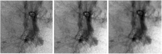
  can be separated in two disjoint regions, the one of which contains the spectral component of the useful signal and, the other, of the noise. We illustrate this apparent property in Fig. 8.1, where in the middle, there is an image corrupted with additive noise, the spectral power of which is concentrated outside the circle
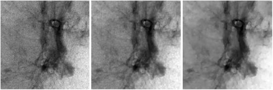
  . On the contrary, the spectral power of the useful signal (left) is concentrated inside this circle. The right image is the convolution of the corrupted image with the ideal filter, i.e., the filter, the transfer function of which is
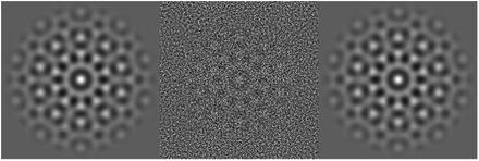
acts upon the image as a local weighted averaging, which is uniform for the whole image and is independent from its current space context. Linear filtering is perfect if the power spectrum of the image can be separated in two disjoint regions, the one of which contains the spectral component of the useful signal and, the other, of the noise. We illustrate this apparent property in Fig. 8.1, where in the middle, there is an image corrupted with additive noise, the spectral power of which is concentrated outside the circle . On the contrary, the spectral power of the useful signal (left) is concentrated inside this circle. The right image is the convolution of the corrupted image with the ideal filter, i.e., the filter, the transfer function of which isFig. 8.1
Linear filtering of the band-limited image. Left: the image the power spectrum of which is inside the circle B. Middle: the same image with added noise, the power spectrum of which is outside the circle B. Right: convolution of the middle image with the ideal filter given by (8.14)
(8.14)
Clearly, in this case, the original image and the denoised one are identical. In fact, if the power spectrum of the useful signal is concentrated inside a bounded region of the frequency domain and the signal-to-noise ratio is big enough in this region, then the linear filtering is still excellent independently from the spectral distribution of the noise. The corresponding example is illustrated in Fig. 8.2. On the left of this figure, there is the same image as in Fig. 8.1 with added white noise and, on the right, the result of the filtering with Gaussian filter  , the transfer function of which is
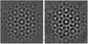
, the transfer function of which isFig. 8.2
Linear filtering of the band-limited image. Left: image from Fig. 8.1 with added white noise. Right: the convolution with Gaussian kernel
(8.15)
Thus, the following short conclusion can characterize the linear filtering: it works well if applied to regular signals, i.e., such signals the power spectrum of which is concentrated within a bounded region of low frequencies and it vanishes fast outside this region. The filtering operation in this case is reduced to the suppression of high-frequency components of the image. If the Fourier transform of an image decays slowly as  , the linear filtering is not efficient anymore. Since the spectral power of such images is high also in the high-frequency sub-band, suppressing within this sub-band affects the sharpness of edges and destroys fine details of the image. This results in overall blurring of the image (see Fig. 8.3).
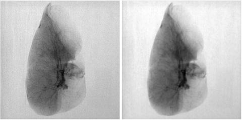
, the linear filtering is not efficient anymore. Since the spectral power of such images is high also in the high-frequency sub-band, suppressing within this sub-band affects the sharpness of edges and destroys fine details of the image. This results in overall blurring of the image (see Fig. 8.3).Fig. 8.3
Blurring effect of the linear filtering. Left: X-ray image of a human lung specimen. Right: convolution with a Gaussian kernel
There is a variety of filters and corresponding smoothing kernels which are available. However, all rely on the same principle and show similar behavior.
8.4 Adaptive Nonlinear Filtering
In contrast to methods based on linear filtering, many advanced noise reduction techniques assume a control over the local amount of smoothing. Appropriately choosing a smoothing kernel at the current positions, it is possible to avoid unnecessary blurring in regions of high variation of the useful signal. Usually in practice the desired kernel is chosen from a predefined family of kernels. As an example we consider the family  , where
and the generating kernel  is a smoothing kernel [see definition above, (8.13)]. It can easily be seen that for σ > 0,
  , that is,
  is also a smoothing kernel. Besides,
  , which implies that
  , where
  is a Dirac delta function. These properties allow to construct the image gF defined by
where we determine  depending on current position
  . The challenging task is to establish a rule according to which the value
  can be adapted to the current context of the image. Usually,
  is required to change as a function of some decisive characteristic such as the gradient, the Laplacian, the curvature, or some other local characteristic of the image. An example of such filtering with the Gaussian function
as a generating kernel, and the squared deviation  as a local decisive characteristic, is given in Fig. 8.4. Particularly for this example, the current value of
  was set to
where
and the function ![$${h_1}:[0,1]\to [0,1]$$](/wp-content/uploads/2016/08/A270527_1_En_8_Chapter_IEq000870.gif) is monotonically increasing from zero to one. For the local squared deviation, we have
is monotonically increasing from zero to one. For the local squared deviation, we have
where the ball  is a ball of radius
  located in
  ;
;  is the local mean value of
  inside the ball.
, where(8.16)
is a smoothing kernel [see definition above, (8.13)]. It can easily be seen that for σ > 0, , that is, is also a smoothing kernel. Besides, , which implies that , where is a Dirac delta function. These properties allow to construct the image gF defined by(8.17)
depending on current position . The challenging task is to establish a rule according to which the value can be adapted to the current context of the image. Usually, is required to change as a function of some decisive characteristic such as the gradient, the Laplacian, the curvature, or some other local characteristic of the image. An example of such filtering with the Gaussian function(8.18)
as a local decisive characteristic, is given in Fig. 8.4. Particularly for this example, the current value of was set to(8.19)
(8.20)
is monotonically increasing from zero to one. For the local squared deviation, we have(8.21)
(8.22)
is a ball of radius located in ; is the local mean value of inside the ball.Fig. 8.4
Filtering with adaptive bandwidth Gaussian kernel. Left: a patch of the X-ray image shown in Fig. 8.3; middle: the result of the filtering by given tuning parameters  and
and  ; right: linear filtering with Gaussian kernel by
and ; right: linear filtering with Gaussian kernel by The smoothing considered in this example incorporates two tuning parameters, which are the constants  and
and  . From (8.19) it follows that
  varies between
  and
and  , and the type of this variation depends on the type of the growth of the function h 1 defined in (8.20).
and . From (8.19) it follows that varies between and , and the type of this variation depends on the type of the growth of the function h 1 defined in (8.20).Another class of smoothing techniques is the so-called sigma filtering. Here we use smoothing kernels of the following general form:

where  is the current update position;
  and
and  are the smoothing kernels, the effective width of which are
  and
and  , respectively; and the local constant
  is determined from the condition
(8.23)
is the current update position; and are the smoothing kernels, the effective width of which are and , respectively; and the local constant is determined from the condition(8.24)
Because of two kernels acting both in the space and the intensity domains, sigma filtering is sometimes referred to as bilateral filtering (see [4]). As it follows from (8.23), the sigma filter is represented by a family of kernels which depends on two scale parameters  and
and  . The parameter
  determines the radius of the ball
  centered in
  . Using the parameter
  , it has to be decided which values
  inside the ball
  have to be weighted down. Normally, these are values which deviate from the value
  . In other words, the kernel
  generates the local averaging mask that allocates those points within the ball
  where image values are close to
  .
.
and . The parameter determines the radius of the ball centered in . Using the parameter , it has to be decided which values inside the ball have to be weighted down. Normally, these are values which deviate from the value . In other words, the kernel generates the local averaging mask that allocates those points within the ball where image values are close to .Bilateral filters are especially efficient if applied iteratively. Denoting the filtering operation with  , the iterative chain can formally be represented as
  .
.
, the iterative chain can formally be represented as .In [5], it has been shown that the best result by an iterative sigma filter can be achieved if  . It can be shown that such a sequence of filtered images converges to the image which is piecewise constant. As an example, in Fig. 8.5, there are three iterations of bilateral filtering where
  and
and  are both Gaussian.
. It can be shown that such a sequence of filtered images converges to the image which is piecewise constant. As an example, in Fig. 8.5, there are three iterations of bilateral filtering where and are both Gaussian.Fig. 8.5
Sigma filtering. Three iterations of applying sigma filter to the patch of the lung phantom
8.5 Wavelet-Based Nonlinear Filtering
A quite different principle for spatially adaptive noise reduction is based on the reconstruction from selected wavelet coefficients. For the sake of completeness, before describing the related techniques, we will review main points of the theory of the wavelet transform referring mainly to [6] and [7]. In doing so, we will use the terminology of the theory of functions, and therefore, we start by stating formal notations accepted in this theory and used in the text.
 ,
,  , is a space whose elements are
  times continuously differentiable functions; the space
  is the space of continuous functions, and
  , the space of piecewise continuous functions.
Let us have  and
and  . As spline space
  , we will call the set of all such functions
  , the restriction of which to the interval
 ![$$ [{2^j}k,{2^j}(k+1)] $$](/wp-content/uploads/2016/08/A270527_1_En_8_Chapter_IEq0008117.gif) is the algebraic polynomial of order
is the algebraic polynomial of order  ; the points
  are called knots of the spline space
  .
.
and . As spline space , we will call the set of all such functions , the restriction of which to the interval is the algebraic polynomial of order ; the points are called knots of the spline space .A space with an inner product  is called Hilbert space. In the following, the norm of element
  is defined by
is called Hilbert space. In the following, the norm of element is defined by(8.25)
 is a space of functions satisfying
  . The space
  is a Hilbert space with the inner product
(8.26)
 is a complex conjugate of
  .
. is a set of all infinite sequences
  such that
  . The space
  is a Hilbert space with the inner product
(8.27)
Span  is the minimal space spanned on the family
  , i.e., for any
  ,
,
is the minimal space spanned on the family , i.e., for any ,(8.28)
Operators that map a Hilbert space  into Hilbert space
  will be denoted as
  . With
  , we denote the adjoint of
  , i.e., such that
  for any
  and any
  . The operator is self-adjoint, if
  .
.
into Hilbert space will be denoted as . With , we denote the adjoint of , i.e., such that for any and any . The operator is self-adjoint, if .A wavelet is a function  that necessarily satisfies the condition
that necessarily satisfies the condition(8.29)
Everywhere in the text, it will be supposed that  is real and normalized, i.e.,
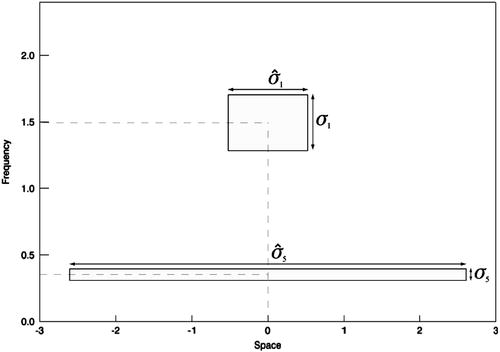
  . Wavelets are “famous” for being well localized both in the space domain and in the frequency domain. The localization properties of wavelets are usually expressed in terms of a so-called space-frequency window. This is a rectangle
  in the space-frequency plane with
  and
and  defined by
is real and normalized, i.e., . Wavelets are “famous” for being well localized both in the space domain and in the frequency domain. The localization properties of wavelets are usually expressed in terms of a so-called space-frequency window. This is a rectangle in the space-frequency plane with and defined by(8.30)
(8.31)
The point  is the center of the space-frequency window of the wavelet. Since
  is real, the modulus of its Fourier transform is even, and this is why the integration in (8.31) is made over the positive half axis only.
is the center of the space-frequency window of the wavelet. Since is real, the modulus of its Fourier transform is even, and this is why the integration in (8.31) is made over the positive half axis only.Wavelet  is called the mother wavelet for the family
is called the mother wavelet for the family (8.32)
 . As an example, let us consider the family generated by so-called Mexican hat wavelet
(8.33)