Fig. 15.1
1D illustration of the spill-in and spill-out effects. The solid blue line represents the true distribution, the dashed blue lines indicate the edges of the target region, and the red line represents the blurred contributions from the target and background regions separately
In order to obtain accurate quantitative values from PET data, it is necessary to correct for a number of physical effects, including random coincidences, electronic dead time, detector efficiency variations, photon attenuation, Compton scattering, patient motion and PVE. Most of these effects are well understood, and correction methods have been developed and are being used routinely. Also PVE is a well-understood effect and a number of correction methods have been developed over the years. However, these are not generally being used routinely. There are several reasons for this: additional data are required, complex image processing is involved, and the result is sensitive to small errors at various stages of processing.
The PVE can be described using the point spread function (PSF) of the system, which essentially corresponds to the image of a point source. The PSF is often characterised mathematically by a Gaussian function, and the amount of blurring is determined by the full width at half maximum (FWHM) of this function. If every point in the actual distribution is blurred by the same amount, then the measured image is described as a convolution between the true image and the PSF. Convolution is a mathematical integral operation between two functions (see, e.g. [1]).
15.1.2 The Partial Volume Effect
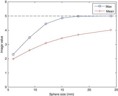
Figure 15.2 shows an illustration of the PVE in 3D. The true object was a cylindrical phantom (20 cm in diameter) containing six spherical inserts (diameters 6, 9, 12, 15, 18 and 24 mm) with a sphere-to-background contrast1 of 4. The phantom was blurred with a 3D Gaussian PSF with a 6-mm FWHM (typical for the resolution of current PET systems). The figure includes cross sections of the original and blurred phantoms, as well as a circular profile through the spheres. In the largest spheres, there is a section where the measured values coincide with the true values. In the smaller spheres, on the other hand, the maximum measured value is reduced in comparison to the true value. There is therefore a limit in terms of object size, above which the measured max value can be used as an estimation of the true mean value (under the assumption that the object is homogeneous and noise-free). In fact, to use the maximum value in a region is one way to mitigate the effect of PVE. This is a simple method that may work for relatively large, uniform objects, although it is very sensitive to noise. The max and mean values in each sphere are shown in Fig. 15.3 as a function of sphere diameter. It can be seen that the point at which the max value starts to drop below the true value is ~3⋅FWHM. The mean value always underestimates the true mean value, but it is less noise sensitive than the max value, and the amount of underestimation can be predicted.
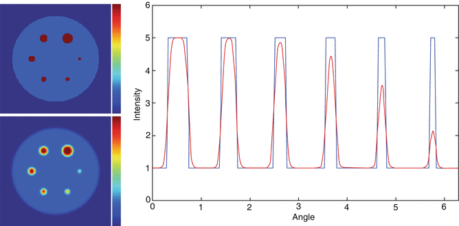

Fig. 15.2
Illustration of 3D PVE. The images on the left hand side show transaxial sections of the original phantom (top) and the blurred image (bottom) (intensity scale, 0–5). The graph on the right hand side shows a circular profile through the spheres. The blue line represents the true data and the red line represents the blurred data
15.1.3 The Point Spread Function
In PET, the PSF can often be modelled as a Gaussian function, and the FWHM is sometimes assumed to be constant over the field of view (FOV). In general, the PSF actually varies over the FOV due to the geometry of the detector system. The resolution is determined by the “tubes of response”, defined by two opposing detectors. The scintillation crystals used in PET scanners typically have a small cross section in order to give high resolution, but are quite long in the radial direction for high sensitivity. This means that, as you move away from the centre of the scanner, the photons can hit the crystals at an oblique angle, leading to what is known as the “parallax effect” and resulting in broadening of the tubes of response and degradation of the spatial resolution (Fig. 15.4a).


Fig. 15.4
PSF variation in (a) PET with a scanner, consisting of a ring of detectors (only a small number are shown), and (b) SPECT using a rotating scintillation camera (The effects have been exaggerated for illustration purposes)
In SPECT, the PSF also varies over the FOV, but for a different reason. The resolution is defined mainly by the geometry of the collimator, resulting in a “cone of response” for a given detector position. This means that the resolution becomes worse with increasing distance from the detector, as the cone becomes wider (Fig. 15.4b). In SPECT, it is easier to model the resolution during forward and back projection, and it can therefore be advantageous to perform PVC during the reconstruction process (see, e.g. [2]). If the image space PSF can be accurately estimated, then post-reconstruction PVC can also be performed in SPECT, using the same methods as in PET.
15.1.4 The Tissue Fraction Effect
PVEs are also said to occur in MRI and CT images. However, in this context, the term does not refer to the effect of the limited spatial resolution of the system, but to the effect of the finite size of the image voxels. Those voxels which are on the boundaries between different organs or tissues would in principle correspond to a mixture of tissue types. We will refer to this sub-voxel effect as the “tissue fraction effect” (TFE). PET images would also be affected by this, but the main cause of PVE in PET is the system PSF. The TFE can usually be addressed to some extent by simply using smaller voxels (although it is arguably always present).
15.1.5 Clinical Implications
In clinical studies, if no correction for PVEs is performed, an implicit assumption is made that the PVE is either negligible or constant in space or in time or across subjects.
In neurological studies, most PET tracers used are primarily taken up in grey matter (GM). The GM layer in the cerebral cortex is only a few mm thick, resulting in a significant amount of PVE. In elderly patients suffering from dementia, there is often a certain degree of atrophy, which further reduces the cortical thickness. In this situation, it is not possible to determine whether a reduction in image intensity is due to reduced tracer concentration in GM or is a result of increased PVE due to reduced cortical thickness.
In cardiac studies, various tracers are used that are taken up in the myocardium. The myocardial wall has a thickness of ~10 mm, but it changes over the cardiac cycle, the wall being thicker at end systole as compared to end diastole. This leads to a change in PVE and, consequently, in image intensity. This “systolic brightening” can actually be clinically useful, as it provides indirect information about the myocardial wall thickening.
In oncology, PET studies are often acquired before and after therapy, in order to monitor the effect of the therapy on the tumour. The follow-up study would typically be done a few weeks after the baseline study, during which time the tumour size may have changed and therefore also the PVE. The change in image intensity will be a combination of both the change in tracer uptake and in tumour size. Reduction in tracer uptake or in tumour size both results in reduced image intensity and is an indication of a positive therapy outcome. Therefore, it is not always considered necessary to correct for PVE in this type of study. On the other hand, it may be more useful to obtain the information about tumour size and tracer uptake separately, rather than as a combined outcome measure, as the change in tumour volume may conceal preserved or incremented activity concentration in a small sub-volume that may merit further treatment.
15.1.6 Partial Volume Correction
Methods to correct for PVE are known as “partial volume correction” (PVC) method, although sometimes the term “partial volume effect correction” has been used. The basic principle behind PVC is to utilise the high-resolution anatomical structural information from CT or MRI data to improve the quality of the PET images, with the assumption that the tracer uptake is controlled by the anatomical boundaries. The anatomical image has to be aligned with the PET image, and it usually also needs to be segmented/parcellated into anatomical regions that can be assumed to be relatively uniform in terms of tracer uptake. PVC methods can be divided into region-based and voxel-based methods, depending on whether they provide only corrected regional mean values or a corrected image. In both cases, anatomical regions need to be defined. A number of PVC methods have been proposed over the years, but we will not attempt to cover all of them in this chapter. Instead, we will primarily focus on the most commonly used methods, but we also will describe some of the more advanced techniques that may have future appeal. A recent review of PVC methods can be found in [3].
15.2 Theory
15.2.1 Deconvolution
As mentioned above, PVEs are caused by convolution of the true object distribution with the system PSF. Therefore, it would seem reasonable to believe that PVC could be performed by an inverse convolution, or deconvolution, procedure. Such a procedure can be implemented either during or after the image reconstruction and can provide a certain degree of resolution recovery, resulting in a reduction of PVEs. However, a full correction cannot be achieved with these methods, partly due to information that is lost and cannot be recovered and partly due to an increased noise level and image artefacts.
Convolution of the true image by the PSF results in an attenuation of mid-range frequency information and a loss of high-frequency information. The former can be restored by various types of deconvolution of inverse-filtering techniques, but the latter can never be recovered from the blurred data. At higher frequencies, the data is usually dominated by noise, and any attempt to restore the high-frequency components will result in noise amplification. Sharp boundaries in images are represented using high-frequency components. If these are lost from the image, any algorithm attempting to restore the sharp boundaries will attempt to do so using components from lower frequencies, resulting in oscillations, with over- and undershoots on both sides of the boundaries. This is the so-called Gibb’s effect.
Since no new information is introduced, deconvolution algorithms can only provide alternative solutions with different resolution vs. noise trade-offs, based on the original data. The procedure is therefore analogous (but with opposite effect) to smoothing with a low-pass filter. These algorithms should be regarded as optional steps in the image reconstruction process and not as PVC algorithms. Here we will use the term “PVC algorithm” only for those algorithms that utilise structural anatomical information from CT or MRI images (sometimes known as “anatomically guided PVC algorithms”). The role of the anatomical data is to provide local high-frequency information, corresponding to anatomical boundaries.
Figure 15.5 shows the effect of applying an iterative deconvolution algorithm [4] to the blurred image from Fig. 15.2. It can be seen that this algorithm results in ring artefacts in the larger spheres, overcorrection at the centre of the medium-size spheres and under-correction in the smallest sphere. For comparison, the image obtained by using the anatomically guided PVC algorithm region-based voxel-wise correction (RBV) [5] is also shown. This image is identical to the original phantom, which shows how powerful PVC, based on anatomical information, can be. It should also be said that iterative deconvolution algorithms can be improved by incorporating so-called edge-preserving smoothness constraints. This corresponds to utilising a priori information about the expected image, assuming that it should be piecewise constant. The information about the location of the edges must, however, be extracted from the PET data itself.


Fig. 15.5
Restoration of the blurred image in Fig. 15.2 using an iterative deconvolution algorithm (left) and an anatomically guided PVC algorithm (right) (intensity scale, 0–6.5)
15.2.2 Motion
Blurring in PET images can also be caused by motion, such as respiratory, cardiac or patient body motion. However, this is a different effect to the blurring caused by the system PSF and should be treated differently. The blurring caused by motion cannot, in most cases, be described by a simple Gaussian function and cannot be assumed to be uniform. There is no way to avoid the PSF blurring, but motion blurring, on the other hand, can be reduced or even eliminated completely by simply using shorter time frames. It then becomes a motion correction problem (see Chap. 16). The two effects are independent and can be treated separately; motion correction should be applied first and then PVC.
15.2.3 Region-Based PVC
We will now describe a series of PVC methods to correct for the system PSF only. (A more detailed mathematical description can be found in the appendix.) Figure 15.6 shows a scheme representing the early developments of PVC methods, including some still commonly used ones. In 1979, Hoffman et al. introduced the term PVE and proposed a method for correcting the mean value in a volume of interest (VOI), assuming a uniform distribution within the VOI and no background activity [6]. The true mean value is obtained by simply dividing the measured mean value within the VOI by a recovery coefficient (RC), precalculated based on the shape and size of the VOI and the system PSF. This method is therefore corrected for spill-out but not for spill-in. Later, Kessler et al. calculated RC values for cases with a non-zero background activity [7]. In this way, correction could be done for both spill-in and spill-out at the same time, but it was necessary to know the true target-to-background contrast in order to select the correct RC values.


Fig. 15.6
Development of traditional PVC techniques
A different approach was chosen by Henze et al. for cardiac studies [8] (see also [9]). They developed a method to correct for the crosstalk between two different VOIs, corresponding to the myocardium of the left ventricle (LV) and the blood pool inside the LV. The contributions from each VOI to the other one and to itself were calculated based on the system PSF. A system of two linear equations was then set up, which could easily be solved by matrix inversion, resulting in the true mean values in the two VOIs.
The same principle was later used by Rousset et al. for neurological studies [10]. In this case, the brain was parcellated into multiple VOIs, based on MRI data. This method can in principle handle any number of VOIs, although the matrix inversion operation can become numerically unstable with too many VOIs. The authors called the crosstalk matrix the “geometric transfer matrix” (GTM), and the method became known as the GTM method. Another method, proposed by Labbé et al., was based on a slightly different formulation with a much larger crosstalk matrix [11]. In the original paper, the authors used an algorithm based on singular value decomposition to calculate the matrix inverse; however, a more practical solution is obtained by using the Moore-Penrose pseudo-inverse instead. The method then becomes very similar to the GTM method. In both cases, the image is parcellated into a number of VOIs. In the GTM method, the image is then sampled using the original VOIs, while in the Labbé method, the VOIs are first blurred by the system PSF. This leads to a different crosstalk matrix, but the output from both methods will be the corrected mean values in the original VOIs. The theoretical difference between these two methods is that the Labbé method in principle utilises all the data corresponding to each VOI in the estimation of their mean values, resulting in a slightly different accuracy vs. precision trade-off.
A simple region-based PVC method was developed by Hofheinz et al. for oncology [12]. It is based on the definition of three regions (VOIs) for each tumour: a target region, corresponding to the actual tumour; a “spill-out” region, surrounding the target region; and a background region, surrounding the spill-out region. First a background term is estimated using the background region and subtracted from the spill-out region. The true activity concentration in the target region is then determined as the total activity in the target and spill-out regions divided by the volume of the target region. The advantage with this method is that it is not very sensitive to an accurate estimation of the PSF.
15.2.4 Voxel-Based PVC
In the methods described above, the image was divided into a number of regions (or VOIs), and the goal of the PVC was to estimate the true mean value within these regions. For voxel-based PVC, it is still (in general) necessary to divide the image into regions, but the correction is then applied to each voxel within these regions separately, thereby producing a new, corrected image. The basic idea is to correct for the spill over from one region to another, but the correction is different for each voxel, as the spill over is not uniformly distributed.
The first voxel-based PVC method was presented by Videen et al. [13]. It was essentially an extension of the Hoffman method. One target VOI was defined and RC values were calculated for each voxel within this VOI, correcting for spill-out but not spill-in. The method was intended for neurological studies and was based on a CT image, segmented into brain and non-brain regions. The brain region included both grey matter (GM) and white matter (WM). This method was later implemented by Meltzer et al. [14], using MRI instead of CT data, and is often cited through this reference.
Later, Müller-Gärtner et al. improved the method by incorporating spill-in correction [15]. In this case, the brain was segmented into three regions: GM, WM and cerebrospinal fluid (CSF). The target region was GM, while WM was considered as a background region. The activity concentration in CSF was assumed to be zero, but it was necessary to know the true value in WM for the spill-in correction. This could be estimated from a WM region, less likely to be affected by PVE. The spill-in from WM to GM was calculated and subtracted, before using the voxel-based RCs to correct for spill-out. This is an additive-multiplicative method, in which PVC is applied to the target region (GM) only.
An alternative approach was used by Yang et al. in their voxel-based PVC method [16]. This method can be seen as an extension of the Kessler method. Multiplicative correction factors are generated for each voxel in the whole image, correcting for both spill-in and spill-out simultaneously. This method requires prior knowledge of the contrast between the different regions. In Yang et al. [16] the method was implemented for brain studies with a 3-class segmentation into GM, WM and CSF, assuming relative activity concentrations of 4, 1 and 0, respectively.
15.2.5 Combined PVC Methods
The PVC methods mentioned above have certain advantages and disadvantages: the region-based methods can only provide mean regional values, while the voxel-based ones require various types of prior information. However, by combining the two approaches, you can get the best of both worlds. Figure 15.7 shows a schematic illustration for how this can be done. The procedure consists of the following four steps:


Fig. 15.7
Schematic illustration of the combination of region- and voxel-based PVC. Region-based PVC is performed first, using VOIs defined in the MRI or CT image and the system PSF. Voxel-based PVC can then be performed, using a piecewise constant pseudo-image, generated based on the corrected VOI mean values, resulting in a corrected image (See text for step-by-step description)
- 1.
The anatomical image is segmented/parcellated into a number of VOIs.
- 2.
Region-based PVC is applied to obtain the mean values in each VOI.
- 3.
A piecewise constant pseudo-image is generated, where all voxels in each region contain the corresponding mean value.
- 4.
The pseudo-image is finally used to perform a voxel-based PVC.
In step 2, either the GTM method or the Labbé method can be used. In step 4, either a Müller-Gärtner-type or a Yang-type correction can be used. Two such algorithms have been proposed: the “multi-target correction” (MTC) method [17] and the “region-based voxel-wise correction” (RBV) method [5]. Another alternative is a method known as “iterative Yang” (iY), proposed in [3], in which the regional mean values are estimated in an iterative procedure with a Yang-type correction, avoiding the GTM step.
Recently a new PVC method was introduced, called “single target correction” (STC) [18]. This method only requires segmentation of the region to be corrected and does not need any a priori information regarding the activity distribution. It operates using region-based spill-out correction and voxel-based spill-in correction, which are applied to both target and background regions.
15.3 PVC Examples
15.3.1 Data Generation
We simulated PET data corresponding to various digital phantoms using the following procedure: (1) the true activity distribution was blurred in the image domain with a 3D Gaussian function with a FWHM of 6 mm, representing the system PSF; (2) the resulting image was forward projected into 180 angles over 180° and multiplied by a forward projected attenuation map; (3) a uniform background was added, representing randoms and scattered events, corresponding to 33 % of the data; (4) the projection data were scaled so as to obtain a realistic total number of counts, and Poisson distributed data were generated using a random number generator; (5) images were reconstructed using FBP, after background and attenuation correction; and (6) the reconstructed images were smoothed with a 3D Gaussian with a FWHM of ~5.3 mm for noise-reduction purposes. For each phantom, the simulations were repeated with 30 different noise realisations.
15.3.2 Example 1: Oncology
We simulated data corresponding to an oncology study using the NCAT torso phantom [19], including respiratory and cardiac motion with periods of 5 s and 1 s, respectively. Data was generated for 40 frames (gates) over one respiratory period. Two spherical tumours (20 mm diameter) were added to the phantom, one in the lung and one in the liver. After reconstructing each frame independently, motion correction (MC) was applied, using an estimated motion pattern. PVC was then applied to each tumour using STC [18].
Figure 15.8 shows a coronal section of the true distribution as well as the reconstructed image without correction, after MC only and after both MC and PVC. Profiles through the tumours are shown in Fig. 15.9, and the mean values in the tumours are presented in Table 15.1, including results obtained with the Hofheinz method [12].


Fig. 15.8
Simulated oncology study. (a) Original phantom (single frame), (b) simulated PET image including motion blurring and PVE, (c) image after MC, (d) image after MC and PVC (STC)
Table 15.1
Quantitative results of the oncology simulation experiment (%, mean ± SD)
Corrections | Method | Lung tumour | Liver tumour |
|---|---|---|---|
Mean ± SD | Mean ± SD | ||
Uncorrected | 46.97 ± 0.34 | 58.49 ± 0.36 | |
MC | 57.22 ± 0.28 | 71.11 ± 0.37 | |
MC + PVC | Hofheinz | 89.75 ± 0.76 | 96.49 ± 1.15 |
STC | 89.79 ± 0.50 | 93.69 ± 0.70 |
In the uncorrected image, the tumours are elongated due to motion blurring. MC restores their round shape and increases the intensity. PVC improves the uniformity in the tumours and further increases the intensity. Quantitatively, the correction is not perfect. This could be due approximations in the motion pattern or in the PSF. The Hofheinz method seems to give slightly higher accuracy than STC in the liver tumour. This could be because it is less dependent on the PSF. However, it relies on a uniform background and does not produce a new image.
15.3.3 Example 2: Cardiology
The same phantom was used as in the previous example, but without tumours. MC was applied and the image frames were merged into eight cardiac gates. PVC was applied to the myocardium using STC [18]. The heart was reoriented into standard short- and long-axis sections.
Images with and without correction are shown in Fig. 15.10 for the end systole (ES) and end diastole (ED) phases of the cardiac cycle, and quantitative results are presented in Table 15.2.


Fig. 15.10
Cardiac phantom for end diastole (left panel) and end systole (right panel) gates, including vertical long-axis (first column) and short-axis (second column) sections. The top row shows true activity distribution with MC; the second row, uncorrected images; the third row, images after MC only; and the bottom row images obtained after MC and PVC (STC)
Table 15.2
Quantitative results from the cardiac phantom simulation experiment
End diastole | End systole | Difference (%) | |
|---|---|---|---|
True values | 100 | 100 | 0 |
Uncorrected | 65.0 | 70.0 | 7.53 |
MC | 75.5 | 78.5 | 3.88 |
MC and PVC | 93.2 | 94.0 | 0.84 |
In the uncorrected images, there is underestimation of the myocardial image intensity, and there is a difference between ES and ED. After MC, the intensity is increased and the ES-ED difference is reduced. After MC + PVC, there is further increase in intensity, and the difference is reduced to <1 %.
15.3.4 Example 3: Neurology
We used a brain phantom [20] for testing several of the PVC methods developed for neurology studies. The phantom contained a number of cortical and subcortical regions (Fig. 15.11). The matrix size was 256 × 256 × 128 and the voxel size 1.1 × 1.1 × 1.4 mm. From the original phantom, we generated a segmented version, containing regions for grey matter (GM), white matter (WM) and cerebrospinal fluid (CSF) (Fig. 15.11), and also an activity distribution, with values of 0.8–1.2 in the GM regions, 0.25 in WM and 0.01 in CSF. A sinusoidal pattern was added to the image, in order to introduce some intra-regional variation (Fig. 15.12). We applied five different PVC methods to the reconstructed image: (1) Videen/Meltzer (V/M) [13, 14], (2) Müller-Gärtner (MG) [15], (3) GTM [10], (4) MTC [17] and (5) RBV [5].

