2.1Musculoskeletal System

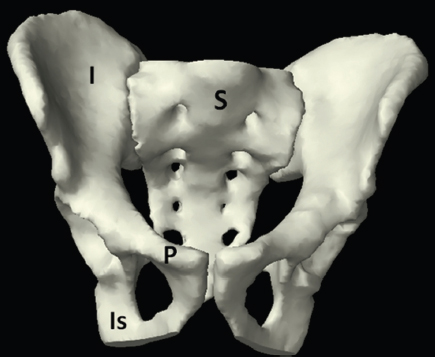
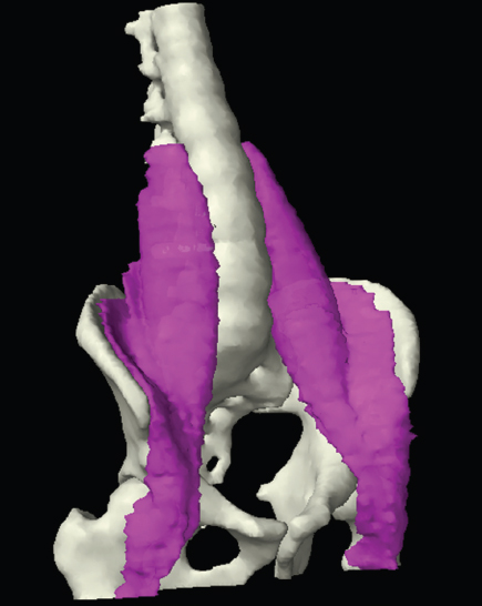
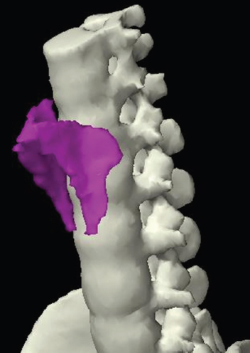
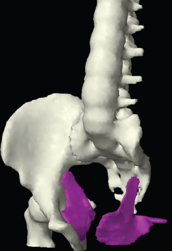
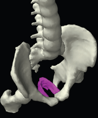
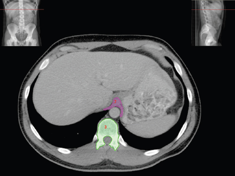
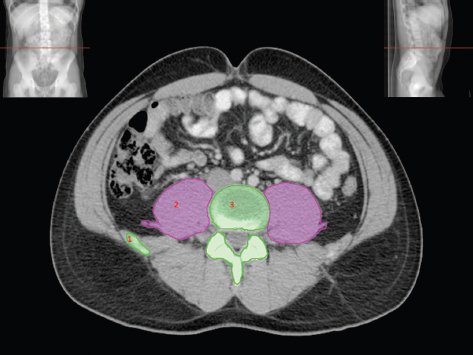
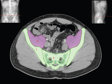
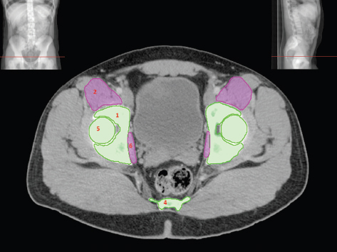
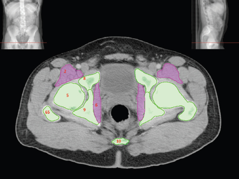
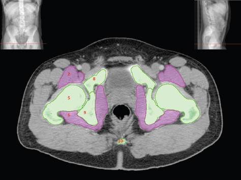
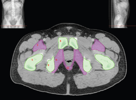
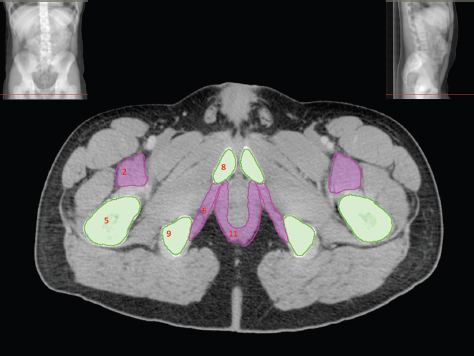
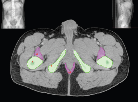
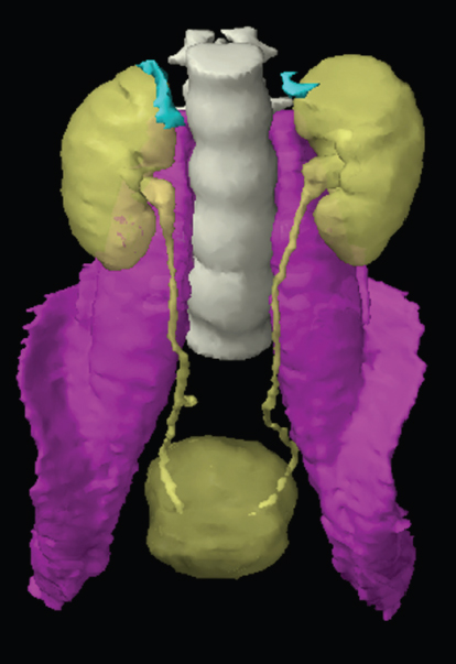
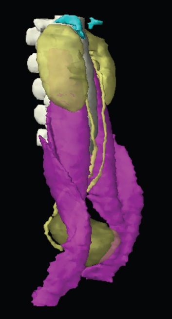
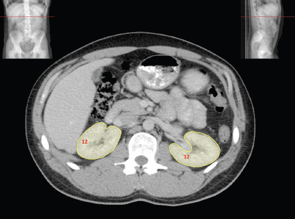
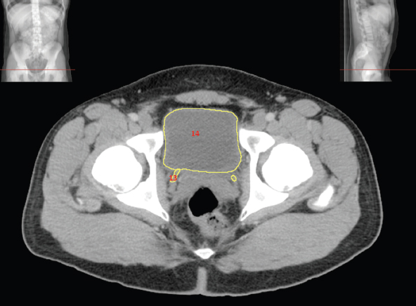
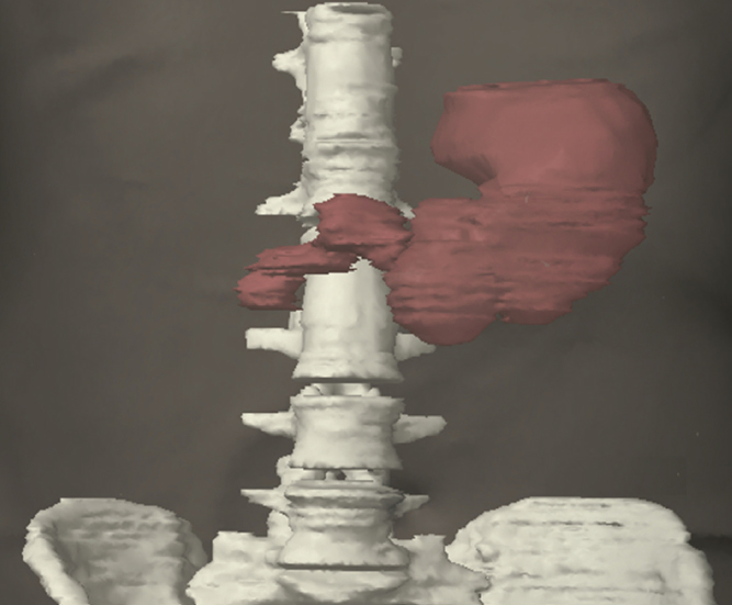
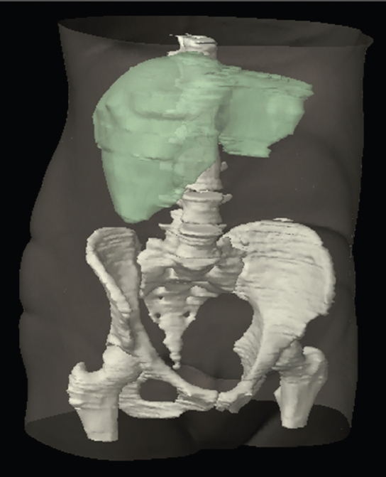
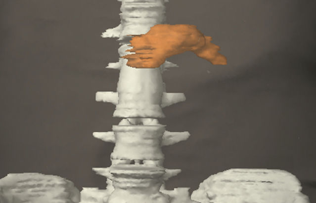
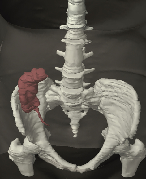
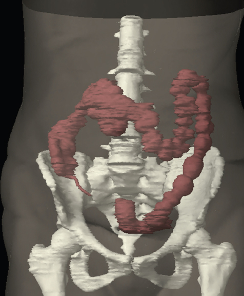
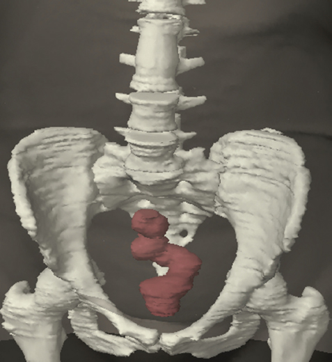
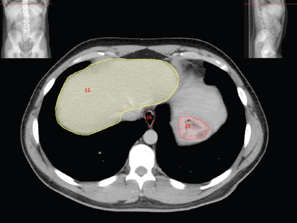
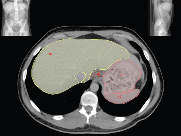
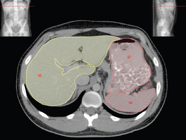
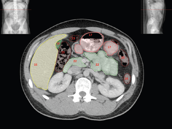
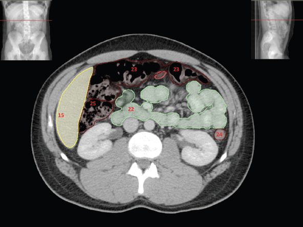
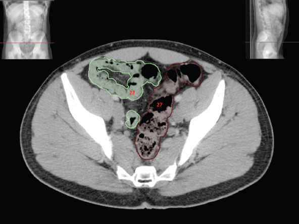
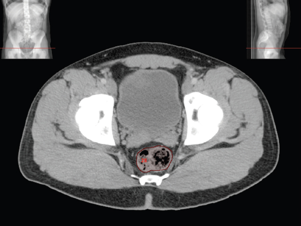
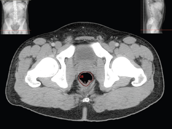
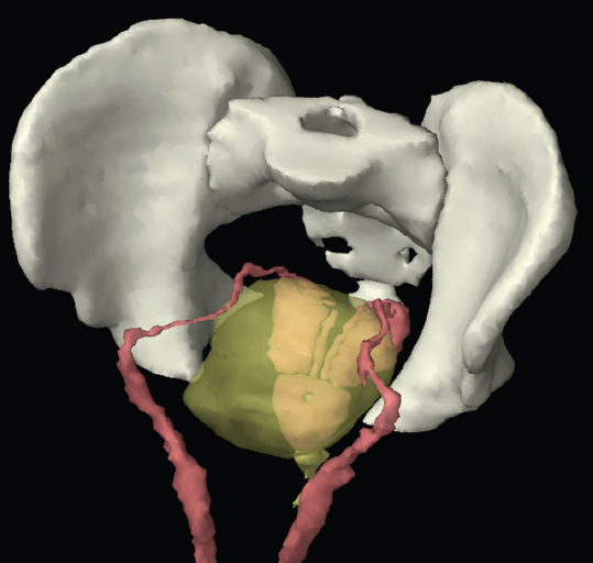
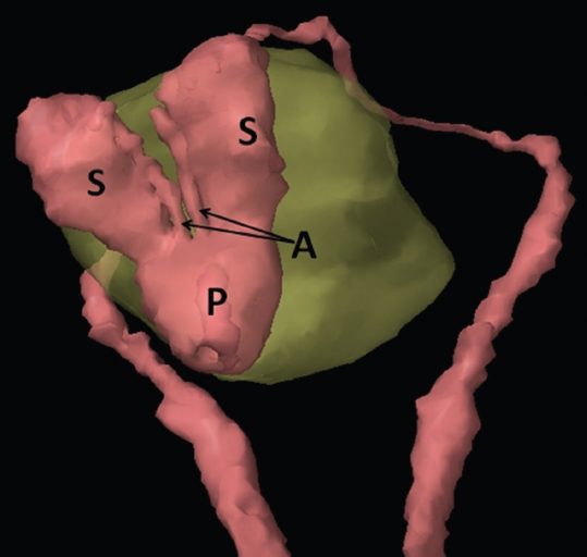
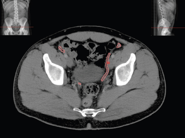
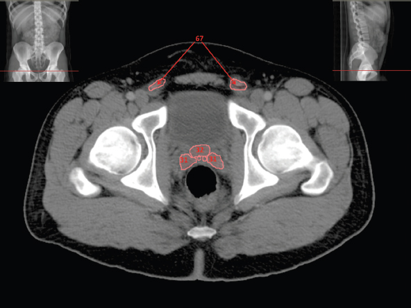
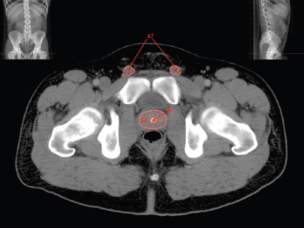
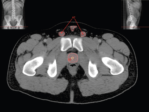
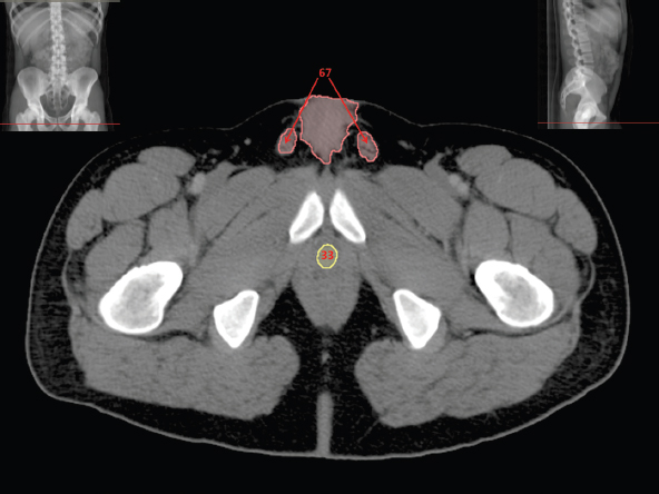
The bony pelvis comprises the sacrum and coccyx at the posterior with the innominate bones forming the lateral and anterior boundaries. Figure 2.1.1 illustrates the relationship between these bones. Each innominate bone is a fusion of three separate bones: the ilium (I), ischium (Is) and pubis (P). The superior and largest component is the ilium. Each ilium has a flared crest on the superior edge and a slightly concave inner surface known as the iliac fossa. The ilia intersect with the sacrum (S) via the sacroiliac joint. This extends for a considerable distance superior-inferior as well as anteriorposterior. The inferior of the ilium forms the superior of the acetabulum.

The acetabulum is the bowl-shaped depression that is the receptacle for the head of the femur. The inferior half of the acetabulum is formed by the ischium posteriorly and the pubis anteriorly. Figure 2.1.1 illustrates the relationship between the three components of the pelvic bones. An essential radiological feature of the pubic bones is the symphysis pubis, the anterior connection between the two rami. The other notable pelvic bony feature is the obturator foramen, which is the aperture formed by the arches of the pubis and the ischium. The skeletal system in the abdomen is much simpler, comprising the five lumbar vertebrae. On CT the wide nature of the vertebral bodies is evident as they are designed to support most of the body’s weight.

The majority of the abdominal muscles are not immediately relevant in common radiotherapy practice since they rarely form target volumes or critical structures. Of note, however, are the paired psoas muscles lying parallel to the vertebral column, anteriorly and laterally, as shown in Figure 2.1.2. The psoas muscles are useful features to identify on CT since the ureters run anteriorly to them. They become wider as they descend the abdomen, joining the iliacus muscle, which covers the iliac fossae. At this point, they are known as the iliopsoas muscles. They then continue and reduce in size inferiorly until they reach the lesser trochanter of the femur.

Towards the superior of the psoas muscles, they are joined by the crura of the diaphragm. The crura are shown extending towards the vertebral column in Figure 2.1.3. The diaphragm constitutes the boundary between thorax and abdomen and the two muscular ‘crura’, or legs, extend inferiorly along the spine to serve as anchors for the diaphragm. The retrocrural space between the crura and the vertebrae contains some important structures as will be seen later.

In the pelvis, some of the muscles should be identified to help distinguish them from other more relevant anatomy. The prime candidate for confusion is a collection of three flat muscles collectively known as the levator ani, as shown in Figure 2.1.4. This sheet runs from anterior to posterior, to form the inferior of the pelvis and thus provide support for the pelvic organs. In the male the proximity of the levator ani can cause confusion when attempting to delineate the inferior aspect of the prostate. Although not outlined in Figure 2.1.4, the levator ani muscle is connected to the coccyx by a fibrous band called the ‘raphe’.

Further support for the pelvic organs is provided by the obturator muscles (Figure 2.1.5). They run along the lateral inner edge of the pelvis, covering the obturator foramina. They form the lateral support for the pelvic organs, forming a ‘basket’ shape with the levator ani muscle. The obturator internus are of note since they help denote the position of the obturator lymph nodes as will be seen later.

Figure 2.1.6 shows how the musculotendinous crura (7) of the diaphragm track posteriorly to meet the anterolateral surfaces of the upper lumbar vertebrae (3). The right crus is usually slightly thicker than the left and the crura in general are thickened anteriorly. The space behind the crura is known as the retrocrural space. It contains fatty adipose tissue in which several other higher attenuation smaller vessels and structures can be seen.

The thick psoas muscles (2) are seen in Figure 2.1.7 lateral to the lumbar vertebrae (3). These are occasionally split into psoas major and minor and are visible on most sections from the mid abdomen to the pelvis. They form part of the posterior abdominal wall and attach proximally to the lateral aspects of the lumbar vertebrae and intervertebral discs from T12 down to L5. They attach distally to the lesser trochanter of the femur. Although measuring about 45HU, similar to adjacent soft tissue structures, the psoas muscles are readily distinguishable on CT cross-section by the surrounding retroperitoneal adipose tissue (-65HU). The tip of the right iliac crest (1) is also seen on this image.

Figure 2.1.8 demonstrates the sharp contrast between the highly attenuating bone of the ilium (1) and the adjacent soft tissue structures, particularly at the cortex where bone density is greatest. The less dense ‘cancellous’ interior is a mixture of bone and fatty marrow organised in a ‘trabecular’ structure and thus appears less dense.

Within the sacrum (4), two sacral foraminae and the vertebral canal are seen. On axial section, the angle of the sacroiliac joints can be appreciated. Within the pelvis in Figure 2.1.8, the psoas muscle is joined by the iliacus muscle arising from the iliac fossa, to form the iliopsoas muscle (2).

More inferiorly, in Figure 2.1.9, the iliopsoas (2) pierces the inguinal canal and is visible anterior to the ilium (1). Although rarely a site of primary pathological process, the psoas and iliopsoas muscles are both clinically and radiologically significant due to their proximity to the aorta, inferior vena cava, kidneys, ureters, digestive tract, pancreas, lymph nodes and spine. In cross-section, the femoral heads (5) appear round, located deep within each acetabulum formed by the ilium (1). The obturator internus muscle (6) is seen on the medial border of the ilium.

Figure 2.1.10 features more of the pelvic bones including the ischium (9) and pubis (8). The pubis (8) forms the anterior pillar of the acetabulum while the ischium (9) forms the posterior column. The obturator internus muscle (6) adjacent to the pelvic wall denotes the border of the pelvic brim, forming the top of the funnel-shaped pelvic diaphragm. Its internal borders, although sheathed in fascia, can be difficult to distinguish more inferiorly due to proximity to other pelvic soft tissues and levator ani muscle groups. The right greater trochanter (65) is apparently floating and not attached to the right femoral head (5). As with all structures, the viewer must scroll superior and inferior to fully appreciate the bony structure and components of the pelvis and hip joints.

In Figure 2.1.11 male pelvic structures are seen adjacent to the anterior ‘belly’ of the obturator internus muscle (6) where it attaches to the pubis (8). The muscle can be seen wrapping around the rear of the ischium (9) and inserting into the femur (5) at the medial greater trochanter surface. The inferior tip of the coccyx (10) is visible just anterior to the natal cleft.

Figure 2.1.12 shows the levator ani (11), composed of the pubococcygeus, iliococcygeus and puborectalis muscles. The intimate relationship of this muscle to the rectum, internal pelvic organs and obturator internus muscle (6) is clear. The obturator internus (6) can be seen to bridge the obturator foramen between the pubis (8) and ischium (9).

With the exception of the bony pelvis and fat within the ischiorectal fossa, all other soft tissues are of similar density at about 40HU. This makes CT outlining of the prostatic apex, vagina and anus quite difficult. This is demonstrated in Figure 2.1.13 where potentially all soft tissues enclosed by the levator ani muscle group appear to form a single soft tissue mass, with few distinguishable markings or borders.

The levator ani muscle group (11) forms the base of the funnel shaped pelvic diaphragm closing the inferior pelvic aperture. The urogenital diaphragm, formed by a thin sheet of striated muscle, is located anterior to the levator ani muscle group. These muscles make soft tissue differentiation in the inferior pelvis particularly challenging in both males and females. This can be improved by supporting the axial CT sections with coronal section imaging using high resolution T2 MR. Central to Figure 2.1.14, the levator ani complex (11) intimately surrounds the anus. Fat within each ischiorectal and ischioanal fossa can be seen laterally to each ischium (9), separated centrally by the natal cleft. The shafts of the femora (5) lie laterally to this and the cancellous bony centres are clearly visible, surrounded by the higher density cortex.

The twin starting points of the urinary system are the kidneys, which are located at the rear of the abdomen, slightly anterior to the psoas muscles and lateral to the vertebral bodies. Each kidney is accompanied by an adrenal gland which is located superiorly and medially. These can be seen in Figure 2.2.1. Recall that the right kidney is the lower of the two due to the volume of liver above it.

The final stage of the ureters’ journey takes them around the posterior edge of the bladder towards the inferior ‘trigone’ area. The bladder is the main organ of interest with regard to radiotherapy in the urinary system. Since the bladder is essentially an elastic-walled bag of urine, it will deform readily around more solid anatomy adjacent to it. Thus it is not uncommon to find two or three separate ‘bulges’ of bladder appearing on CT slices around other structures. For some treatments such as prostate, it is common for the bladder to be maintained at full capacity and in these cases the pressure can give the bladder a more consistent shape, although the paler muscular wall stretches thin. For other treatments, such as to the bladder, voiding is encouraged before treatment or imaging. In these circumstances the muscular wall is much thicker but the shape and volume of the bladder can be surprisingly variable.

Urine is produced in the kidneys by filtering out waste products from the bloodstream. The urine collects in the renal pelvis at the centre of the kidney. From here, the urine passes into the ureters. These are long and take an often tortuous route through the abdomen. It can be difficult to pick out the ureters on individual slices, especially with non-contrast images where they can mimic blood vessels. For much of the route, the ureters overlie the psoas muscles, being anterior and slightly medial to them. Figure 2.2.2 shows the ureters curving anteriorly before plunging posteriorly once they pass the fifth lumbar vertebra.

Figure 2.2.3, at L2, shows the left renal hilum complete with renal arteries and veins. In Figure 2.2.4 at a slightly lower level, the ureters (13) have emerged from the renal pelvis.

Demarcation of the kidneys (12) (approx 30HU without IV contrast) is relatively straightforward due to the fibrous capsule and surrounding contrasting ‘perinephric’ fat. The thin layer of ‘Gerota’s’ renal fascia can sometimes be seen surrounding the fat. The adrenal glands, not demonstrated here but discussed later, sit within Gerota’s fascia, superior to the upper poles.

IV contrast enhances the renal cortex in Figure 2.2.4 with the cortical columns of Bertin separating the medulla into pyramid-shaped segments. At the apex of each medullary pyramid, renal calyces form multiple funnellike structures that drain into the renal pelvis. Approximately 60–70 seconds after injection, the renal cortex will enhance (approximately 140HU) and then, minutes later, contrast will fill the renal calyces, renal pelvis, ureters and bladder.

Figure 2.2.5 illustrates the ureters. These are thin fibromuscular tubes of varying diameter (3–7mm). Localisation of the ureters can be complicated, particularly without IV contrast. It is, however, possible to delineate them on CT since they lie within fatty and connective tissues along their entire course. Care should be taken not to confuse ureters with small vessels or fatty stranding.

Ureters are best identified by tracking them inferiorly from the renal pelvis to the bladder. The ureters descend inferiorly and slightly medially from the renal pelvis, towards the anterior surface of the ipsilateral psoas muscle as seen in Figure 2.2.5.

Both ureters descend anterior to each psoas muscle until they cross the pelvic brim where they follow the path of the common iliac artery (Figure 2.2.6).

They then track posteriorly, crossing anterior to the external iliac artery before passing obliquely through the urinary bladder (14) wall posteriorly as seen in Figure 2.2.8. Any obstructive or compressive lesion at any point during the course of the ureter will cause dilation above it (hydro-ureter).

The urinary bladder (14) has variable appearances and position within the pelvis dependent upon the degree of filling. Partially distended bladders can be easily compressed by adjacent structures such as enlarged prostatic lesions, vaginal tumours, other pelvic masses or loops of sigmoid colon, as demonstrated in Figure 2.2.7, indenting the bladder’s anterior right border. A prostatic or uterine fundus ‘impression’ is relatively normal. The partial volume effect is common where, due to its deformable nature, it may look as if bowel loops appear inside the urinary bladder.

When fully distended, the muscular wall should be uniform, smooth, free of calcification, and between 1mm and 3mm thick, measuring approximately 45HU.

After voiding, the urinary bladder walls will appear thicker, and more irregular. Pelvic irradiation will cause uniform inflamed thickening of the bladder wall that will be evident on follow-up planning CT.

Food enters the abdomen via the oesophagus before collecting in the stomach on the left hand side of the body, as seen in Figure 2.3.1. Like the bladder, the stomach is designed to enlarge to accommodate changes in capacity. Thus, unless the patient is undergoing strict dietary control, the stomach can exhibit a wide range of sizes. Immediately after a hearty meal, the stomach will have expanded inferiorly, anteriorly and medially, pushing other structures aside in order to accommodate its contents. On CT, the stomach contents can be seen to exhibit a horizontal fluid level.

After exiting the stomach, the digestive tract forms the duodenum and performs a tight U-turn (Figure 2.3.1), passing inferiorly and then medially to enter the jejunum.

As it does so, it passes under the liver. The liver is a large solid structure dominating the right hand superior portion of the abdomen (Figure 2.3.2). It is the largest gland in the human body and comprises two main lobes, the small left lobe and the larger right lobe. The right lobe contains other much smaller lobes known as the caudate and quadrate lobe. The liver is not a major source of primary tumours but, due to its rich blood supply, it is a common site for metastatic deposits to grow. Sitting under the liver is the pear-shaped gall bladder which stores bile to assist with fat emulsification. Its fluid-filled nature means that on CT it can be readily identified as a darker, less dense structure.

The small intestine then curls round the head of the pancreas. The pancreas can be seen shaded orange in Figure 2.3.3 (from the superior) and Figure 2.3.4 (from the anterior). It lies across the upper abdomen with the tail on the left side, the body centrally placed and the head tucked into the curve of the duodenum. It lies against the spleen posterolaterally and the stomach superiorly.

The small intestine is the next stage of the digestive tract and is a highly mobile structure. It has a sausage-like appearance on CT and can be distinguished from the large bowel by the lack of air in it. In the lower right of the abdomen, the small intestine connects to the large bowel via the ileocaecal valve. The large bowel starts with the caecum. This receives the small intestine contents and is situated in the inferior right hand side of the abdomen. Extending from the inferior part of the caecum is the small useless appendix, occasionally curling to resemble a pig’s tail. The appendix can be seen in Figure 2.3.5 extending inferiorly and medially from the caecum. After exiting the caecum, the ascending colon passes superiorly until it reaches the liver. The colon can be identified by its characteristic appearance of interconnected rounded chambers called saccules.

The ascending colon then bends at the hepatic flexure to form the transverse colon. As the name suggests, the transverse colon moves transversely across the top of the abdomen. It does sag somewhat, however, and thus can loop a considerable distance inferiorly, occasionally causing confusion at lower slice levels as seen in Figure 2.3.6. However tortuous a route it takes, it approaches the spleen and the stomach and turns at the splenic flexure.

From this bend, the descending colon drops down the left hand side of the abdomen until it reaches the sigmoid flexure where it turns into the sigmoid colon as seen in Figure 2.3.7. The sigmoid colon is responsible for moving the intestinal contents from the left hand side of the body to the centrally and posteriorly placed rectum and it does this by forming a characteristic ‘sigma’ shape. The final bend in the digestive tract is the acutely angled rectosigmoid junction, marking the superior border of the rectum. It is important to identify this junction when outlining the rectum as a critical structure to ensure a clinically useful dose-volume histogram can be produced.

The rectum has a different appearance from the colon, lacking the saccules and forming a single large cavity (Figure 2.3.8). The variation in size and shape of the rectum is well-documented and a major cause of uncertainty in reproducibility of pelvic setups. The rectum curves along the anterior surface of the sacrum before moving slightly forward towards the centre of the pelvis. The rectum ends in the sphincter muscles of the anus. The anus is embedded in the levator ani muscle sheet and thus can be identified at the level where the levator ani widens on CT. This occurs because the levator ani is crossing at a more oblique angle along the width of the slice.

In Figure 2.3.9 at T11/12, structures within both the thoracic and upper abdominal cavities are present. In axial cross-section, the soft tissues of the thin muscular diaphragm (45HU) are poorly differentiated against the adjacent liver (15) and stomach wall (17). The crescent-shaped lower lobes of each lung are clearly seen, visually very black and demonstrating few lung markings on this soft tissue window.

In the centre of Figure 2.3.9, immediately anterior to the aorta, is a section of the distal third oesophagus (16). In this case it is slightly dilated, with intraluminal air forming a natural inherent negative contrast agent. The thickness of a healthy oesophageal wall should not exceed 3mm when dilated. Wider circumferential dilatation is usually indicative of pathological or inflammatory process.

The oesophagus does thicken, however, as it passes through the diaphragmatic oesophageal hiatus to join the stomach (17) at the gastro-oesophageal junction (16 in Figure 2.3.10). This may mask the presence of small adenocarcinomas, although they are usually quite advanced and commonly demonstrate irregular luminal narrowing and wall thickening.

Water is also commonly utilised as a negative contrast agent when imaging the distal oesophagus and stomach to demonstrate wall thickening and irregularities. In radiotherapy, the stomach commonly contains partially digested food, as can be seen on Figures 2.3.10 to 2.3.14. The heavier stomach contents sink posteriorly, adjacent to the spleen (56), with fluid sitting on top. Fluid levels with a pocket of air/gas on top, as seen in Figures 2.3.11 to 2.3.14, make the stomach (17) readily distinguishable in many instances.

The pancreas (21) is level with L1/L2 and can be seen extending across the upper abdomen in Figures 2.3.12 and 2.3.13. Its ‘head’ sits right of midline within the curvature of the duodenum (20) while its body and tail extend to the left, posterior to the stomach and just anterior to the splenic vein. The CT appearance of the pancreas becomes less smooth and more lobulated with age, although increased fatty deposits make it easier to locate.

The liver (15) occupies a large part of the upper abdominal cavity in the right upper quadrant, as can be seen in Figures 2.3.9 to 2.3.16. The four lobes are divided by fissures meeting at the porta hepatis, where the portal vein enters the liver. The right lobe is the largest, occupying most of the right hand side. The left lobe, separated from the right by the falciform ligament, extends to the left across the midline in many instances. The caudate lobe is the smallest, and can be seen in Figure 2.3.11 immediately anterior to the inferior vena cava (IVC). Inferior to the caudate, the quadrate lobe lies behind the gall bladder.

The gall bladder (19), seen in Figures 2.3.12 to 2.3.14, indents onto the quadrate lobe and is dark due to the presence of biliary fluid. The visceral surface of the left lobe of the liver is in contact with the stomach (17), as seen in Figures 2.3.12 and 2.3.13.

Beyond the stomach, the remaining sections of the gastrointestinal tract can be seen on most cross-sections through the abdomen and pelvis, demonstrated in Figures 2.3.11 to 2.3.22.

The duodenum (20) appears in Figures 2.3.12 and 2.3.13, running from the gastric pylorus of the stomach to the proximal jejunum, forming a C-shape around the head of the pancreas (21). As it curves it passes the quadrate lobe of the liver (15), gall bladder (19) and hepatic flexure of the colon (25).

The remainder of the small bowel (22) is composed of jejunum and ileum. These can be seen folding and curving throughout the mid abdomen and pelvis within the peritoneum. As the small bowel is from 3 to 7 metres long, it appears on most abdominal CT sections, as seen in Figures 2.3.14 to 2.3.19.

Generally, the loops of small bowel occupying the left mid abdomen can be identified as jejunum, and loops within the pelvis and right lower abdomen are the ileum. The jejunum is often empty as its Latin name suggests (jejunus means empty). Thus intraluminal detail can only be identified by CT contrast agents.

There are finer radiological identifiers, such as the high concentration of circular folds (plicae circulares) in the proximal jejunum. These increase intraluminal surface area and cause a ‘feathered’ appearance, particularly when positive oral contrast agent is used, as seen in Figures 2.3.14 and 2.3.15. The concentration of these folds gradually decreases along the length of the small bowel and they are absent at the terminal ileum.

The change in intraluminal CT appearance is evident in Figure 2.3.16 where there is a distinct difference between the much smoother appearance of the ileum to the right of midline, compared to that of the jejunum, left of midline. As the intraluminal contents are usually more fluid in consistency, any pockets of air will normally rise to the anterior aspect of the lumen, assuming the patient is supine, as can be seen clearly in Figures 2.3.18 and 2.3.19.

The large bowel or ‘colon’ can also be seen throughout the abdomen and continues into the pelvis. It can be traced through Figures 2.3.11 to 2.3.22 (18, 23, 24, 25, 27, 28 and 66). The CT appearances of the colon can be distinguished from loops of the small bowel by larger folds and the presence of intraluminal gas within solid faecal matter.

The colon usually follows a relatively simple and less tortuous route when compared to the small bowel. The ascending colon rises on the right (25) before turning at the hepatic flexure (61). The transverse colon (23) crosses the abdomen to the left, then turns at the splenic flexure (18) to form the descending colon (24) dropping down the left side.

After the sigmoid flexure, the sigmoid colon (27) curls around into the pelvis before forming the rectum (28) and anus (29). It is useful to follow this route superior and inferior on contiguous CT slices when attempting to visualise the different parts of the colon. To trace the path of the colon, it is often easier to start at the rectum (28 in Figure 2.3.20). The rectum may be easier to locate on axial CT slices than the caecum (66 in Figure 2.3.17).

Figure 2.3.20 shows the rectum quite loaded with faecal matter and gas. Surrounding the rectum, the dark layer of fat within the perirectal fascia provides a boundary between the rectum and adjacent structures. Scrolling superiorly from the rectum, the sigmoid colon (27 in Figure 2.3.19) extends anteriorly across the left piriformis and iliopsoas muscles and iliac vessels towards the left anterior abdominal wall. The descending colon, surrounded by fat (24 in Figures 2.3.13 to 2.3.17), can be traced up from the pelvic brim to the splenic flexure (18 in Figure 2.3.12).

At this point it is important to scroll inferiorly and superiorly to trace the transverse colon (23) to the right, posterior to the anterior abdominal wall. The path of the transverse colon is quite tortuous as it often sags inferiorly. At the hepatic flexure the ascending colon (25) can be traced inferiorly down to the blind ended caecum (66 in Figure 2.3.17) at the ileocaecal valve. The vermiform appendix (26) can be seen lateral to the caecum, in the right iliac fossa.

Returning to the rectum, in Figure 2.3.21 the rectum (28) has a large pocket of intraluminal gas visible. This is clearly pushing the other pelvic organs anteriorly, demonstrating the difficulty presented by variable rectal volume when attempting to localise target positions.

The walls of the rectum should be about 5mm thick. Posteriorly to the rectal wall can be seen the striations of the coccygeus muscle (part of the levator ani complex). These lie within the ischiorectal fossae and extend laterally to the lateral pelvis walls. They should not be mistaken for rectal wall.

In Figure 2.3.22, the muscular walls of the anus (29) can be seen centrally, surrounded by the levator ani complex.

The essential function of the internal reproductive system of the male is to produce and combine the various ingredients of semen. Sperm cells are transported inside the body from the testes via the vasa deferentia. These paired tubes run up the outside of the pelvic wall inside the spermatic cord, along with the testicular artery and vein. They then penetrate the abdominal muscles through the inguinal canal and leave the spermatic cord. Figure 2.4.1 shows how the spermatic cords are thicker than the vasa deferentia. Each vas deferens then loops its way posteriorly, curving over the top of the bladder as seen in Figure 2.4.1. They then descend the posterior wall of the bladder and approach each other, widening out to form an ‘ampulla’ each.

The main component of semen is seminal fluid, which is produced and stored in the seminal vesicles. They are long feathery structures that extend superiorly and slightly laterally along the posterior wall of the bladder and are a common site for spread of prostate tumours. The seminal vesicles (S) and ampullae (A) join up superior to the prostate (P) as seen in a view from the inferior and posterior in Figure 2.4.2. Together they form the ejaculatory ducts which then descend to penetrate the prostate gland.

The prostate gland sits under the bladder, encircling the urethra, and is the size and shape of a walnut. It is responsible for adding prostatic fluid to the sperm and seminal fluid. The ejaculatory ducts carry the fluid anteriorly to join the urethra inside the prostate.

The urethra then exits the prostate gland, passes through the small and often indistinguishable bulbourethral or ‘Cowper’s’ gland for its final ingredients and then passes down the penis superiorly to the penile bulb. The penile bulb is the proximal section of the penis, between the two roots of penis.

Figure 2.4.3 shows the vasa deferentia (30). They are a pair of 3–5mm thick muscular tubes following a tortuous route from the testes to a dilated ampulla at the base of the seminal vesicles (31 in Figure 2.4.4). As such, they can be quite difficult to locate and track along their course. Knowledge of their course and adjacent anatomy can help the viewer track them, and as with all tubular structures on CT, it is essential to view contiguous slices superiorly and inferiorly along their course.

Each vas deferens (30) ascends from the scrotum, within the spermatic cord (67), external to the pelvic cavity, seen on Figures 2.4.5 to 2.4.10. The spermatic cord is a little easier to localise, since it is larger and contains the vas deferens, testicular artery, vein, lymphatic ducts, nerves and surrounding fatty tissues.

Passing through the inguinal canal, as seen in Figure 2.4.4, the vasa deferentia leave the spermatic cords and enter the pelvic cavity. From here, they cross over the external iliac vessels and between the supero-lateral borders of the bladder and the lateral pelvic wall. This section of the left ductus is seen in Figure 2.4.3 (30).

The duct then crosses the posterolateral angle of the bladder, traverses the ureter, and can be seen in Figure 2.4.4, medial to the seminal vesicles (31). At this point, the vasa deferentia are easier to demarcate due to ampullary dilatation.

Figure 2.4.5 shows the paired seminal vesicles (31) located between the base of the urinary bladder and the rectum. These are lobulated soft tissue structures and are not fixed. They can appear asymmetrical, but tend to resemble a bow-tie, extending either side of the vasa deferentia ampullae, as seen in Figure 2.4.4.

More inferiorly, the prostate gland (32) can be seen in Figures 2.4.6 to 2.4.8. Sitting inferior to the neck of the urinary bladder and level with the symphysis pubis, the prostate encloses the urethra (33). It is pyramidal in shape, with its base in contact with the bladder and apex resting on the pelvic floor muscles. A normal prostate measures around 40mm LR, 30mm AP and 50mm SI. The size of the gland is dependent on age and after 45 years gland enlargement is not uncommon. As a consequence, the gland often indents into the bladder.

On CT, the prostate appears relatively homogeneous, with a soft tissue density of approximately 50HU. The prostate’s zonal anatomy is often indistinguishable. Prostatic secretions can sometimes cause flecks of calcification within the gland. Ring-like calcifications are occasionally seen, although these tend to be associated with previous infection. The borders of the healthy gland are smooth and can be well demarcated in some individuals by surrounding fat deposits. The prostate is also surrounded by a rich plexus of vessels and nerves. Anteriorly, this is termed ‘the anterior plexus of Santorini’. Posterolaterally (at 5 and 7 o’clock positions) this plexus is known as the neurovascular bundles. This periprostatic plexus can cause confusion when attempting to identify and outline the inferior border of the gland. Calcified ‘phleboliths’ within these venous vessels peripheral to the gland can help to identify the capsule.

Related posts:

CT in Radiotherapy Introduction Thorax Intracranial Head and Neck (Extracranial) Transtrochanteric Curved Varus Osteotomy for the Treatment of Osteonecrosis of the Femoral Head

Stay updated, free articles. Join our Telegram channel

Join