PET Image Reconstruction: Methodology and Quantitative Accuracy

Fig. 11.1

One ring of a typical PET scanner and data processing

In modern PET scanners, the septa were removed for 3D data acquisition to improve the system sensitivity. For 3D PET, the data can be stored either as projections indexed by (x _r, y _r, θ, ϕ) or equivalently as stacks of sinograms indexed by (s, ϕ, z, θ), as shown in Fig. 11.2. Data on 3D PET scanners are typically stored in the stacked sinogram format and sometimes compressed by adding the neighboring angles or sinograms together.

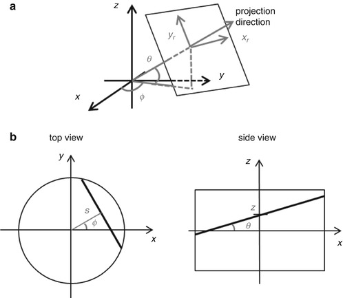
Fig. 11.2

3D PET data stored in (a) projection and (b) sinogram format

11.2.2 Filtered Backprojection

11.2.2.1 Line Integral Model and Central Slice Theorem

A simple model for PET data assumes that the number of events detected at each detector pair is proportional to the integral of the radioactivity along the line connecting the centers of the two detectors. This is the basis upon which analytic image reconstruction algorithms are developed. Here we illustrate the line integral model for the 2D case.

Mathematically, the spatial distribution of the tracer is represented by a 2D continuous function f(x,y). Measured projection data can then be approximated by the discrete samples of the x-ray transform of f(x,y), which is defined by

$p\left(s,f\right)=\underset{-\infty }{\overset{\infty }{{\displaystyle \int }}}f\left(s \cos f-t \sin f,s \sin f+t \cos f\right)dt$

(11.1)

where s is the distance of the projection line to the center and ϕ is the projection angle, as shown in Fig. 11.2b.

An important result that underlies analytic image reconstruction is the central slice theorem. In 2D, the central slice theorem relates the 2D Fourier transform of the image to the 1D Fourier transform of its x-ray transform p(s, ϕ), as illustrated in Fig. 11.3:

Fig. 11.3

2D central slice theorem

$F\left({\omega}_s \cos f,{\omega}_s \sin f\right)=P\left({\omega}_s;f\right)$

(11.2)

where the 1D and 2D Fourier transforms are defined by

$\begin{array}{l}F\left({\omega}_x,{\omega}_y\right)={\displaystyle \int \int }f\left(x,y\right){e}^{-2\pi i\left({\omega}_xx+{\omega}_yy\right)} dxdy\hfill \\ {}P\left(\omega \right)={\displaystyle \int }p(s){e}^{-2\pi i\omega s}ds\hfill \end{array}$

(11.3)

This relationship shows in 2D that the Radon transform uniquely describes any Fourier transformable image and that the image can be reconstructed by forming its 2D Fourier transform according to (Eq. 11.2) and taking an inverse 2D Fourier transform. Although this is a straightforward way of reconstructing 2D images, it requires the interpolation of the image’s 2D Fourier transform onto a rectangular grid, and reconstructed image quality depends on the accuracy of the interpolation. As a result, direct Fourier reconstruction methods are not commonly used.

11.2.2.2 Backprojection Filtering

An image can be formed by integrating all the projections passing through a point and assigning the value of the integral to the point. This linear operation is called backprojection and can be expressed mathematically as:

$b\left(x,y\right)=\underset{0}{\overset{\pi }{{\displaystyle \int }}}p\left(x \cos f+y \sin f,f\right)df$

(11.4)

It can be shown that this backprojected image corresponds to the original image smoothed by the “1/r” blurring in Fourier transform domain:

$B\left({\omega}_x,{\omega}_y\right)=F\left({\omega}_x,{\omega}_y\right)/\sqrt{\omega_x^2+{\omega}_y^2}$

(11.5)

In order to recover the original image f(x), we can filter this backprojected image, and the overall approach is known as backprojection filtering (BPF). A common approach is to switch the order of the linear backprojection and filtering operations and to apply filtering to the 1D projection data (usually by convolution with the filter function in projection space) before backprojection, thus called filtered backprojection or FBP [4]. As shown in (Eq. 11.5), the reconstruction filter has a frequency response of |ω|. This so-called ramp filter amplifies high-frequency noise; therefore, in practice, a windowed ramp filter is used in FBP reconstruction and frequency components above a threshold (cutoff frequency) are set to zero. Frequently used window functions in 2D FBP include Shepp–Logan, Butterworth, and Hann windows [5, 6]. Figure 11.4 shows FBP images of a simulated NCAT phantom using different window functions.

Fig. 11.4

Images reconstructed from simulated NCAT phantom (a) noiseless and (b) noisy data. Top 4 rows were reconstructed using Butterworth window with orders 2, 4, 8, and 32, respectively. Bottom row used Hann window. Left to right: cutoff frequencies of 0.1, 0.2, 0.3, 0.4, and 0.5 cycle/pixel, respectively (Reproduced from Tsui and Frey [6])

11.2.3 Reconstruction of 3D PET Data

The 2D central slice theorem can be extended to 3D PET, resulting in the derivation of 3D FBP [7]. However, due to the limited axial coverage of PET scanners, not all oblique projections are recorded, and therefore some oblique projections through the imaging volume are missing. As a result, a typical 3D PET scanner corresponds to a shift–variant system where FBP cannot be directly applied to reconstruct the data. Figure 11.5 shows a direct line of response (LOR) which is acquired in 2D PET, an oblique LOR acquired in 3D PET and a missing oblique LOR in 3D PET that is not measured because the LOR does not intersect the detector surface.

Fig. 11.5

Cross section of a PET scanner: events along LOR1 is acquired in 2D PET, LOR2 is acquired in 3D PET, while LOR3 is missing from the 3D PET data

One solution to the missing data problem is to estimate the truncated projections before applying 3D FBP. The 3D reprojection (3DRP) algorithm was proposed to estimate the missing data and has been a standard analytic reconstruction algorithm for 3D PET [8]. In 3DRP, unmeasured data is estimated by calculating the line integrals along the LORs through an initial image estimate obtained by applying 2D FBP to the non-oblique sinograms.

We note that 3DRP is based on the fact that 2D data is sufficient for reconstruction (e.g., 2D images reconstructed from line integrals on parallel planes can be stacked to form the final 3D image), and the goal of using additional 3D data is to improve the statistical properties of reconstructed images. While 2D and 3D reconstructions would be identical for reconstructions from noiseless data, at typical clinical data noise levels, by including the events detected by two detectors on different rings, 3D reconstructions significantly improve the signal-to-noise ratio (SNR) of the image.

Another way to reconstruct 3D PET data is to explore the redundancy in the data and to reduce it to a 2D dataset. Such a process is called rebinning. Since the computational cost of rebinning is negligible compared to the computational cost of image reconstruction, the resulting reconstruction speed is almost the same as that of 2D reconstructions.

A simple way to rebin 3D PET data is through the process called single slice rebinning (SSRB) [9] where a stack of 2D sinograms are created by placing detected events on the plane perpendicular to the scanner axis (z) and lying in the middle of the line connecting the two detectors that detected the event. Mathematically we have

$p\left(s,f,z\right)={\displaystyle \sum}_{\frac{z_1+{z}_2}{2}=z}p\left(s,f,{z}_1,{z}_2\right)$

(11.6)

where s and ϕ are the coordinates of the line of response projected onto the x–y plane and z ₁ and z ₂ are the location of the two detector rings (z ₁ may equal to z ₂).

SSRB is only accurate when the activity is concentrated near the axis of the scanner. In cases of extended activity distributions, such as whole-body FDG scans, SSRB will become less accurate and introduce distortions. A more accurate rebinning method called Fourier rebinning (FORE) has been developed based on the relationship between the Fourier transforms of the 2D data and oblique data [10].

Following SSRB or FORE, a 2D reconstruction algorithm is applied to reconstruct each slice separately. The advantage of FORE is that it allows fast 2D reconstructions while retaining the SNR benefits from 3D data. Figure 11.6 shows a brain FDG scan data reconstructed using 3DRP and FORE + FBP. The image quality is comparable while the speed of FORE + FBP is more than ten times faster than 3DRP.

Fig. 11.6

A central transaxial slice of an FDG brain scan reconstructed using (a) 3DRP and (b) FORE + FBP [10]

Although FORE has been widely used for clinical 3D PET image reconstruction, it is still based on the line integral geometric model and cannot model all the physical effects in PET data acquisition. In addition, FORE requires all the data corrections to be applied directly to the data (instead of being part of the system model), and therefore changes data noise properties which become difficult to model when a 2D iterative algorithm is used to reconstruct the rebinned dataset. As a result, fully 3D statistical reconstruction methods are preferable over FORE rebinning followed by 2D reconstruction methods.

11.3 Model-Based Statistical Reconstruction

Analytic image reconstruction methods inherently assume that noiseless line integrals of the image are available. In reality, data acquired in typical PET scanners are not exact line integrals, and there is significant statistical noise in almost all clinical datasets. Model-based statistical image reconstruction approaches are preferable due to their ability to model the physics and statistics of the imaging process and have become widely available in all commercial scanners. In this section, we first introduce statistical noise models for PET data and physical system models which describe the complex physics of data acquisition. We then review the methodology of maximum likelihood (ML) and maximum-a-posteriori (MAP) estimation and numerical optimization algorithms used to generate PET images. Due to the nonlinear, shift-varying and high-dimensional nature of statistical reconstruction algorithms, image resolution and noise analyses are complicated and are still an active research area. We will give a brief review on this topic in the end.

11.3.1 Noise Model

PET data is inherently noisy, and this fact has significant effects on reconstructed image quality. Statistical reconstruction algorithms model the noise in PET data explicitly and use iterative numerical optimization algorithms to solve the associated optimization problem. Over the last four decades, many model-based statistical image reconstruction algorithms have been proposed. Although the formulae of these methods are quite different, they are all designed to solve the following problem:

$y=\overline{y}(x)+\mathrm{noise}$

(11.7)

where y is the measured data, $\overline{y}$ denotes the mean of the data, and x is the image of the unknown activity distribution. The number of events detected at a detector within a given time due to the radioactive decay inside the object can be accurately modeled by the Poisson distribution:

$P\left(n\Big|\lambda \right)=\frac{e^{-\lambda }{\lambda}^n}{n!}$

(11.8)

where n is the number of decays and λ is the mean, which is equal to the variance.

If system dead time and detector pileup effects are ignored, then measured data can be modeled as independent Poisson random variables with joint distribution:

$P\left(y\Big|\overline{y}\right)={\displaystyle \prod}_{i=1}^M\frac{e^{-{\overline{y}}_i}{{\overline{y}}_i}^{y_i}}{y_i!}$

(11.9)

where y _i is the number of events detected in the ith LOR, ${\overline{y}}_i$ is the mean number of events in the ith LOR that can be calculated using the system model described in the next section, and M is the number of LORs.

While a Gaussian noise model may be used for low-noise data with acceptable accuracy, resulting in the weighted least square (WLS) approach for image reconstruction [11], most statistical approaches use the Poisson model.

In PET, a common practice is to subtract an estimate of the random events (e.g., using delayed window method) online to reduce the bandwidth needed for data transfer and storage space [12]. In that case, measured data at the ith LOR is given by

${y}_i={p}_i-{r}_i$

(11.10)

where p _i is the number of prompts and r _i is the number of delayed events for the ith LOR. While both p _i and r _i are independent Poisson random variables, the difference between the two is no longer Poisson. The distribution of y _i has a numerically intractable form. One can use Gaussian distribution as an approximation to the true distribution of the precorrected data. Yavuz and Fessler noticed that a simple but good approximation is to add $2{\overline{r}}_i$ to the data [13], where ${\overline{r}}_i$ is the mean of the delayed events estimated from the data and to model the resulting random variable as Poisson with mean and variance equal to ${\overline{y}}_i+2{\overline{r}}_i$ .

As we discussed previously, Fourier rebinning is commonly used to reduce the size of the dataset and reconstruction time. It has been shown that FORE rebinned data is no longer Poisson [14]. Similar to the approach for random precorrected data, Liu et al. used a simple scaling to match the mean and variance of the rebinned data [15]. Then a reconstruction algorithm based on the Poisson noise model can be used to reconstruct the resulting data.

11.3.2 System Model

The spatial resolution of PET is limited by several factors such as positron range, photon noncollinearity, and penetration and scattering of the photon in the detector. One critical limitation of analytic reconstruction methods is that these factors are neglected in the simple line integral model. With model-based statistical reconstruction, we use a system model to account for these resolution-deteriorating effects. Other factors may also be included in the system model such as the attenuation of the photons in the body, nonuniform efficiencies of the detectors, and random and scattered events.

In the absence of noise, we can model the data as a linear function of the image:

${\overline{y}}_i={\displaystyle \sum}_{j=1}^N{p}_{ij}{x}_j+{\overline{r}}_i$

(11.11)

or in matrix format $\overline{y}=Px+\overline{r}$

where $\overline{r}$ is the sum of mean of random and scattered events and P is the system matrix, which relates the image to the noiseless data, and can be expressed in factored form as [16]:

$P={P}_{\mathrm{norm}}{P}_{\mathrm{blur}}{P}_{\mathrm{attn}}{P}_{\mathrm{geom}}{P}_{\mathrm{range}}$

(11.12)

where P _range models the blurring due to positron range in image space [17, 18]; P _geom is the geometric projection matrix containing the geometric detection probabilities for each voxel and detector pair combination; P _attn is a diagonal matrix with attenuation factors; P _blur models the blurring in sinogram space due to photon pair noncollinearity, intercrystal penetration, and scattering; and P _norm is a diagonal matrix with normalization factors.

Matrix–vector multiplications with P and P ^T(called forward and backprojection operations) are typically the most computationally intensive components of statistical reconstructions. Over the last decade, considerable amount of research has been done to speed up statistical reconstruction by reducing the time of forward and backprojections. Many algorithms have been developed that explore the symmetry of the scanner geometry [19] or use fast processors such as graphic processing units (GPUs) to achieve high performance at low cost [20].

It has been shown that the modeling of sinogram blurring is important for resolution recovery [16]. The central component of resolution recovery is the estimation of detector point spread functions (PSF). Such PSFs can be calculated analytically [21], estimated from Monte Carlo simulations [16], or measured from point source data [22, 23]. PSF kernels can either be estimated and stored nonparametrically [23], or the PSF measurements can be fit to a given model, such as asymmetric Gaussian functions [22], and the resulting model parameters can be stored. It has also been shown that for Fourier rebinned data, PSF kernels can be estimated from point source data [23, 24].

Another recent trend is to use an image-space PSF model to account for all resolution degrading effects in the imaging process:

$P={P}_{\mathrm{norm}}{P}_{\mathrm{attn}}{P}_{\mathrm{geom}}{P}_{\mathrm{psf}}$

(11.13)

The image-space PSF P _psf can be estimated from an initial reconstruction of point sources without any resolution recovery and is easy to implement as an image-space blurring operation. Recently shift–variant PSFs have been designed to model the degradation of image resolution toward the edge of the field of view (FOV) [25].

Figure 11.7 shows a Hoffman brain phantom data reconstructed with and without PSF modeling. The PSF image shows better resolution and contrast.

Fig. 11.7

Hoffman brain phantom reconstructions for various numbers of iterations. Upper images are transaxial views, and the lower images are sagittal views. PB parallel-beam, non-PSF [22]

One caveat of PSF modeling is that it can result in edge artifacts that have been shown to overestimate activity by up to 40 % in phantom studies [26]. Methods to mitigate edge artifacts include filtering [27] and under-modeling the PSF kernels [28]; however these approaches come at the expense of reduced resolution recovery.

11.3.3 Maximum Likelihood Estimation Methods

Once we have the noise model and system model, statistical methods can be used to estimate the image. Maximum likelihood (ML) is a widely used statistical estimation method and has been applied to PET image reconstruction.

The likelihood function of the data is the probability of observing the data given the image. Usually the logarithm of the likelihood function is used for easier calculation because the logarithm is a one-to-one monotonic function:

$L(x)= \log \left(\mathrm{Prob}\ \left(y\Big|x\right)\right)$

(11.14)

ML estimation seeks the image that maximizes the log-likelihood function:

${\widehat{x}}_{ML}= \arg \underset{x\ge 0}{ \max }L(x)$

(11.15)

The nonnegativity constraint is due to the fact that the concentration of radioactivity is not negative.

The log-likelihood function under the Poisson noise model is given by (omitting the y _i! term which does not depend on x)

$L(x)={\displaystyle \sum}_{i=1}^M{y}_i \log {\overline{y}}_i(x)-{\overline{y}}_i(x)$

(11.16)

ML estimation is a classic optimization problem, where the cost function (or objective function) is the log-likelihood function (Eq. 11.16). There are many numerical algorithms that can be used to find the ML estimate of the image, such as coordinate ascent or gradient-based methods. One of the earliest approaches used for ML PET image reconstruction is the expectation–maximization (EM) algorithm [29]. EM is a general framework to compute the ML solution through the use of “complete” but unobservable data and is composed of two steps. The first step, called the E-step, involves the calculation of the conditional expectation of the complete data, and the second step, called the M-step, maximizes this conditional expectation with respect to the image. In PET, a very common choice for complete data is the number of events detected by the ith LOR that are emitted from the jth voxel. Shepp and Vardi first applied EM to emission image reconstruction [30], and Lange and Carson extended the work to transmission image reconstruction [31].

The update equation of EM algorithm for emission image reconstruction is given by

${\widehat{x}}_j^{k+1}=\frac{{\widehat{x}}_j^k}{{\displaystyle \sum}_{i^{\prime }}{P}_{i^{\prime }j}}{\displaystyle \sum}_i{P}_{ij}\frac{y_i}{{\displaystyle \sum}_{j^{\prime }}{P}_{i{j}^{\prime }}{\widehat{x}}_{j^{\prime}}^k}$

(11.17)

where y _i is the number of events acquired in the ith LOR, P _ij is the element in the system matrix P described in the previous section, and ${\widehat{x}}_j^k$ is the estimate of the jth image voxel at the kth iteration.

The EM algorithm is usually initialized using a uniform image. A new image is then calculated using Eq. 11.17. This process is repeated until a certain number of iterations are reached. Typically a smoothing filter is applied afterward to reduce image noise.

It is interesting to note that the EM update equation can be derived in several ways. One approach is based on using the concavity of the Poisson log-likelihood function and Jensen’s inequality [32]. In another work, Qi and Leahy showed that that EM algorithm is a functional substitution (FS) method [33]. FS is based on designing a surrogate function at each iteration which is easier to maximize than the original function. Under suitable conditions (equal function value and gradient with current estimated image, surrogate function always higher than the original function), it can be proven that the FS method converges to the maxima of the original function [34–36].

It has been shown that EM converges monotonically to the global maximum of the log-likelihood function and the image is guaranteed to be nonnegative if initialized with a nonnegative image [37]. These nice properties made EM a popular algorithm but unfortunately EM converges very slowly. Hundreds or thousands of iterations are usually necessary to ensure the convergence of EM. Hudson and Larkin observed that the convergence of EM algorithm could be significantly speeded up by dividing the projection data into nonoverlapping blocks, or subsets, and applying EM to each subset of the data [38] and named this method ordered subsets EM (OSEM).

OSEM can speed up the reconstruction almost linearly as a function of number of subsets in early iterations. As a result, it has been widely used in clinical PET and SPECT. The speedup of OSEM can be explained in part by viewing EM as a preconditioned gradient-ascent method:

${x}^{k+1}={x}^k+D\left({x}^k\right)\nabla L\left({x}^k\right)$

(11.18)

where D(x ^k) is a diagonal matrix with ${D}_{jj}={x}_j^k/{\displaystyle \sum}_i{p}_{ij}$ and $\nabla L\left({x}^k\right)$ denotes the gradient of the log-likelihood calculated at the kth iteration image. When the image is far away from the solution, the gradient computed from a subset of the data provides a satisfactory direction for increasing the log-likelihood function value [39].

Although OSEM is fast in the beginning, it is not guaranteed to converge to the ML solution, and the convergence depends on the selection of the subsets. In the original OSEM paper, subsets are chosen such that the detection probability of each voxel is equal for each subset, which is called subset balance. It has been proven that with consistent data and under the condition of subset balance, OSEM converges to the ML solution [38]. In practice subset balance is difficult to achieve due to differences in sensitivity and attenuation. A common practice is to choose the projections in each subset with maximum angular separation to avoid directional artifacts. Another OSEM algorithm convergent with consistent data is rescaled block-iterative EM (RBI-EM), in which the OSEM equation is written in gradient-ascent form and a voxel-independent scaling factor is used to avoid the requirement of subset balance [40].

In general PET data is not consistent due to noise, in which case OSEM usually enters a limit cycle [39]. One way to make OSEM converge with noisy data is to reduce the number of subsets: however convergence is then slowed down. Alternatively, we can use OSEM in the earlier iterations and switch to a convergent algorithm in later iterations [41].

Among other ML estimation approaches, Browne and De Pierro proposed a row-action maximum likelihood algorithm (RAMLA) [42], where the stepsize η _k at the kth iteration satisfies the following conditions:

$\underset{k\to 0}{ \lim }{\eta}_k=0,{\displaystyle \sum}_{k=0}^{\infty }{\eta}_k=+\infty$