Figure 1.1 illustrates the generation and propagation of a sound wave. When a molecule is made to oscillate around its resting phase, the oscillation is transmitted to a neighboring molecule in the medium, from this to the next molecule and so on. In this way energy of motion, transmitted from molecule to neighboring molecule, spreads in sinus waves through the medium. This continuous propagation of the energy of motion is called a wave or sound wave. It results in alternating compression and rarefaction in the medium. The atoms and molecules can oscillate along or across the direction of propagation. Hence we can distinguish between longitudinal waves (in the direction of propagation) and transverse waves (across the direction of propagation). Only longitudinal waves can be propagated in gases and fluids, because sound waves lack the shear force necessary for transverse transmission. Physically, biological tissue can be viewed as a viscid liquid. The stronger the cohesion between the molecules, i.e., the denser the material, the greater is the velocity of sound within the material. Table 1.1 provides an overview of the densities of various tissues and the sound velocities within these tissues.

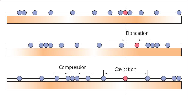
Fig. 1.1 Generation and spread of a sound wave.

The distance between two maximal compressions is the wavelength λ. The number of oscillations of a molecule in unit time is the frequency f, which is measured in hertz (Hz). Their depth of penetration and resolution capacity are listed in Table 1.2. One hertz is a single oscillation per second, i.e., 1 Hz = 1/s. Figure 1.2 provides an overview of the frequency range of sound waves and their applications. Ultrasound waves in the frequency range of 2–30 MHz are used for diagnostic medical imaging.

The velocity of a wave is determined by the product of its wavelength and frequency:

In medical diagnostic imaging the velocity of sound is assumed to be independent of tissue, namely a constant quantity of 1540 m/s.

The displacement of an individual molecule from its resting point in diagnostic imaging amounts to about 2 × 10^-6 mm (0.000002 mm). The pressure of sound waves is typically 0.6 × 10⁵ Pa. At this pressure each oscillating molecule accelerates appreciably to the order of 10⁵ times gravitational acceleration.

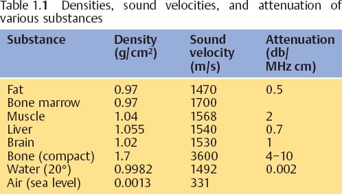
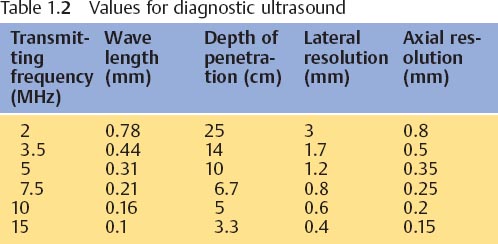
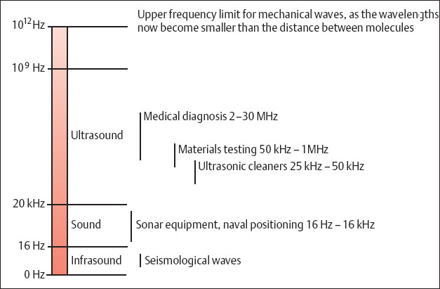
Fig. 1.2 Frequency ranges of sound waves and their applications.

The Generation of Ultrasound

Ultrasonic waves can be generated in a variety of ways, the mechanical method being the simplest. Sounding a tuning fork of less than 2 mm generates ultrasonic waves with a frequency up to 200 kHz. For engineering use such as cutting, drilling, or milling of very small parts (e.g., to divide semiconductors) ultrasound is generated by magnetostriction. In this method a ferromagnetic substance is placed in a magnetic field with alternating polarity, generating frequencies of up to about 50 kHz at considerable sonic intensities.

In 1880 the Curies discovered the piezoelectric effect, which is used for the generation of ultrasonic waves in medical diagnostic imaging. If pressure is exerted on an ionic crystal and an elastic deformation in a defined direction is then imposed on the crystal, the internal charge shifts. Electric potentials result on its surface, negative on one side, positive on the other. The voltage increases as the pressure increases. If, conversely, an electric potential is applied to the surface of a piezoelectric crystal, the latter will become elongated or shortened according to the direction of the voltage. If an alternating potential is applied, the crystal begins to oscillate. Quartz and tourmaline are especially active piezoelectric substances. The piezoelectric materials used to build current ultrasonic probes are made of scintered ceramic such as barium titanate. Figures 1.3 and 1.4 show an electronmiscroscopic image of such a piezoelectric ceramic and a schematic view of the multilayered arrangement used in its structure.

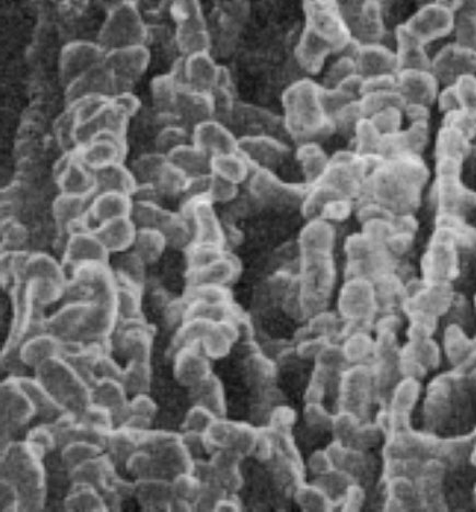
Fig. 1.3 Electronmiscroscopic photograph of a piezoelectric ceramic.

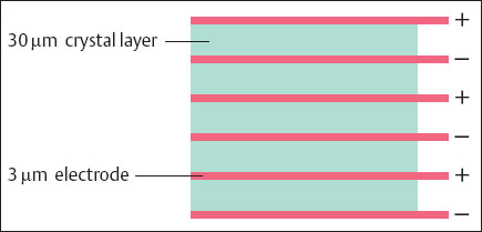
Fig. 1.4 Diagram of the multilayer structure of a piezoelectric ceramic.

Physical Effects

Reflection and Refraction

The propagation of sound in tissue follows the laws of optical waves. At the interface between two tissues of different densities there is a sudden change in impedance. Impedance is defined as the resistance Z to sonic waves, calculated by the product of sound velocity × density. At such an acoustic interface, part of the incident sound wave is reflected (reflection), while another part is refracted and continues into the tissue (transmission) (Fig. 1.5). When the incidence of the sound wave on an interface is vertical, the reflection gradient (R) is calculated by the formula:

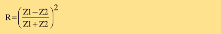
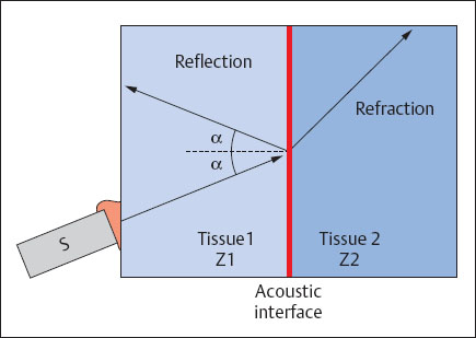
Fig. 1.5 Reflection and transmission of a sound wave at an acoustic interface (S = transducer; Z = impedance).

As a rule the surfaces separating tissues are not smooth but rough or diffuse. Sound waves are not reflected directionally at diffuse interfaces but are scattered in the form of a spherical wave (Fig. 1.6). Tissue structures smaller than the wavelength cause mainly scatter. Tissue structures exceeding the wavelength cause reflection. Scatter echoes generate the typical textured pattern of parenchymatous organs.

Interference

When two or more sound waves arrive at the same time, two waves in different phases may meet (i.e., the compression phase of one wave may coincide with the rarefaction phase of the other), and they may weaken each other. Similarly, waves in the same phase may coincide and reinforce each other. This phenomenon is called interference, and the spatial distribution of areas of weakening and reinforcement are called interference patterns. Interference patterns significantly determine the appearance of an ultrasound image.

Diffraction

When the straight propagation of a sound wave is impeded, for example, by the edge of an object, the wave is bent (diffracted) around such an edge. Thus the sound waves reach the space behind the object, which would normally lie in its shadow (Fig. 1.7).

Absorption

The energy of a sound wave diminishes in the direction of its propagation. The internal friction of the oscillating molecules is transformed into heat, i. e., the sound wave is absorbed. The values of attenuation listed in Table 1.1 may be roughly averaged to 1 dB/(MHz cm). Absorption is dependent on frequency. On the one hand, high ultrasound frequencies are useful because their short wavelengths provide precise localized resolution; on the other hand, it is also necessary to examine organs lying deep below the surface, and for this examination lower ultrasound frequencies with their longer wavelengths are more suited because they attenuate less. At a frequency of 10 MHz the attenuation is 10 dB/ cm; at a frequency of 3 MHz the attenuation is 3 dB/cm. Assuming an initial output of 100 dB, the depth of penetration at a frequency of 10 MHz can be calculated to be 5 cm (10 cm total path) and at a 3 MHz frequency the penetration would be 17 cm (33 cm total path).

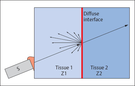
Fig. 1.6 Spherical scattering of a sound wave at a diffuse interface (S = transducer; Z = impedance).

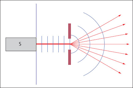
Fig. 1.7 Diffraction of a sound wave at a diffracting edge (S= transducer).

Generating the Image

Pulse-Echo Procedure

Almost all ultrasound procedures used in medical diagnosis are based on the so-called pulse-echo procedure. A brief electrical impulse is applied to the piezoelectric crystal of the transducer, and this impulse is transformed into an ultrasonic pulse by the piezoelectric crystal. The duration of the pulse is about 1 μs. The transducer is then switched to act as a receiver. The sound wave penetrates the tissue and is reflected from the internal boundary interface. The part of the sonic pulse returning to the piezoelectric element is called an echo; it elicits an electric impulse in the element. The time differences between the emission of the ultrasonic pulse and the reception of each echo are then measured. The product of the ultrasound velocity c and the time difference t gives the distance z covered by the ultrasonic pulse. Dividing this number into 2 gives the exact position of the reflecting structure with respect to the transducer:

For a time difference of, for example, 0.13 ms calculation shows a distance of 10 cm between transducer and reflector. Depending on the construction of the transducer, 3000–5000 ultrasonic pulses a second may be emitted. At the same time echoes are captured, calculated, and transformed into images.

Time Gain Compensation

Because some of their sound is absorbed, energy (amplitude) from echoes traveling over a longer period of time from deeper tissues is lower than that of echoes with shorter travel times. Thus, interfaces having equal reflection gradients will emit signals of different amplitudes according to their depth. To equalize the representation of signals, those received at the element after a longer travel time are proportionally amplified. Such amplification is known as time gain compensation (TGC), or depth gain compensation (DGC), and can be controlled by the user of the ultrasound apparatus.

A-Mode

The simplest and also the oldest imaging procedure used in diagnosis is the A-mode procedure. The amplitudes of the electric signals generated at the transducer are displayed on a cathode ray oscilloscope, proportional to the distances of the boundary surfaces in the tissue being examined (Fig. 1.8). Because it represents amplitude, this procedure is known as amplitude mode, or A-mode. A-mode procedures provide only one-dimensional information. Today they are still used in ophthalmology (to determine the thickness of the cornea) and otorhinolaryngology (for noninvasive examination of the nasal sinuses).

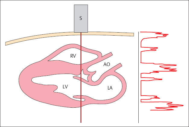
Fig. 1.8 A-mode scan. The amplitude of the electric signals generated at the transducer are displayed on a cathode ray oscilloscope.

S = transducer

RV = right ventricle

LV = left ventricle

AO = aorta

LA = left atrium

In contrast to A-mode, in this procedure amplitudes are represented not as deflections (peaks) but as bright spots on a monitor. The brightness steps of these spots are proportional to the amplitudes of the electric signals and hence those of the echoes. The stronger the signal, the brighter is the point on the image. This procedure is known as brightness mode, or B-mode. In current ultrasonic systems about 256 degrees of brightness can be represented in shades of gray (grayscale display), though the human eye can only distinguish 80 shades of gray. The individual brightness spots are arranged in a straight line, and the sound beam is now shifted before sending a new pulse. If the new lines acquired by this procedure are displayed corresponding to their localization, a two-dimensional cross-sectional image is obtained (Fig. 1.9). 0.2 ms are needed to display a line at a depth of, for example, 15 cm (cf. Pulse-Echo Procedure). For the display x of a width of 5 cm, an interval between lines of Δx of 1 mm, and the known ultrasound velocity c of 1540 ms^–1, the scan time T of 10 ms can be obtained by the formula:

From this may be calculated a repetition frequency for the image of 100 Hz, i.e., 100 separate images per second. It is therefore practicable to generate an image in real time.

M-Mode

In contrast to B-mode display, in M-mode (motion mode), the sound beam is not shifted, but is kept in a fixed position over the organ to be examined. The individual lines are again displayed side by side on a time axis. By this means it becomes possible to visualize movements as they occur in the imaged tissue (Fig. 1.10). At a depth of 15 cm of the displayed tissue the scan time is 0.2 ms, i. e., an image can be generated about 5000 times a second. Thus, even very rapid movements, for example, of the heart valves can be displayed. Since the scales of the image and of the time axis are known, movements, velocities, and acceleration can be accurately measured. Hence M-mode is of great value in echocardiography.

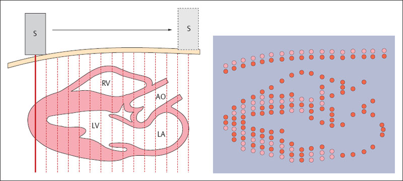
Fig. 1.9 B-mode scan. Generation of a two-dimensional cross-sectional image. S = transducer, RV = right ventricle, LV = left ventricle, AO = aorta, LA = left atrium

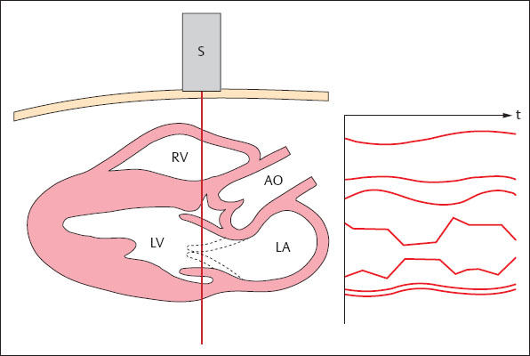
Fig. 1.10 M-mode scan. The course of movements in the insonated field is displayed as it develops over time.

S = transducer

RV = right ventricle

LV = left ventricle

AO = aorta

LA = left atrium

The Sound Field

Resolution

Resolution describes the smallest interval between two structures that allows them to be displayed on the monitor as two distinct objects. Resolution is measured in millimeters. Axial resolution in the direction of the sound beam must be distinguished from lateral resolution, which occurs in a plane at right angles to the axis of the sound beam (Table 1.2). Axial resolution is determined by the pulse length of the ultrasound beam. It usually measures one or more wavelengths. Higher resolution can be attained by using higher ultrasound frequencies with their shorter wavelengths. However, as demonstrated when discussing absorption (p. 6), the penetration of ultrasound diminishes with increasing frequency. Hence it is not possible to avoid the use of lower frequencies to display deeper tissue structures. Lateral resolution is determined by the width of the ultrasound beam, i. e., it is proportional to the diameter of the sound beam. Figure 1.11 is a schematic representation of a simple ultrasonic transducer. The sound field is composed of a narrow focused near field and a divergent far field. Precise scanning is only possible in the focused near field. To improve the resolving power of the ultrasonic beam it must be focused.

Focusing

An ultrasonic beam can be focused in various ways. The simplest is the use of an acoustic lens (Fig. 1.12), since essentially the physical laws of wave optics are valid for the spread of sound (cf. Reflection and Calculation, p. 5). Hence the ultrasonic beam is maximally focused at a fixed point. This point is known as the focal point. The element may be given a concave shape. This is known as internal focusing and is used in the single element systems of mechanical sector scanners.

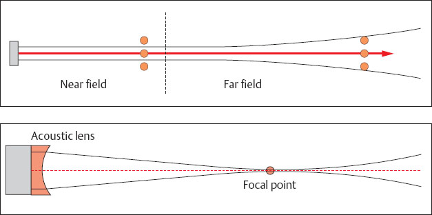
Fig. 1.11 Diagram of the sound field of a simple ultrasonic transducer.

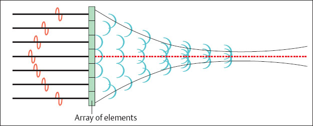
Fig. 1.13 Generation of a concave wave front by time delay of individual crystal elements in an array.

The ultrasound beam is focused electronically in order to reach as variable a depth of focus as possible. Current ultrasonic transducers are built in the form of arrays, consisting of a greater number of individual elements arranged next to each other. The total number of individual elements amounts to between 60 and 256, according to the type of transducer. Several of these individual crystal elements are grouped together to send and receive ultrasound rays. A concave wave front can be generated by regulating the timing of individual elements in the group (Fig. 1.13). Such a wave front converges to a focal point. A sound beam generated in this way is maximally focused at this point and provides high lateral resolution. The focal length can be shifted by varying the width of a group and the timing of the elements. In this way the user can set the focus and with it the point of maximal resolution to the area of diagnostic interest. In modern ultrasound systems it is possible to set several such transmission foci simultaneously. It should be noted that this requires that each sound beam must be repeated for each focal length, and this reduces the repetition frequency of the image. The focusing of the received beam has a special feature: Since the echoes from deeper regions at the transducer arrive later than those from closer regions it is possible in practice to let the receiving focus shift to the deep area. This procedure is known as dynamic receiving focusing. The groups used for focusing vary in width between 8 and 128 elements.

Scanning Procedures

Principle of Operation

The principle of operation of modern scanners is shown in Figure 1.14. As described above, several individual elements in an array are grouped together to generate an ultrasound beam. Such a group generates an ultrasound pulse and also receives the returning echo signals. When an element on the left side is switched on, while an element on the right side is switched off, the new group of elements generates another ultrasound ray that has been shifted by the width of one element. The linear density can also be increased by varying the breadth of the group: First a group of elements generates an ultrasound pulse, then one element, for example, on the left side, is switched off, while on the right none is switched on. The axis of the next ultrasound beam is now shifted relative to the previous group by the width of half an element. If, now, an element on the right side is switched off, while none is activated on the left, the number of lines of sight has been increased by a factor of 2. On the other hand, the time required to scan a complete image increases, i.e., the image repetition frequency is halved. Various scanning devices are described in what follows.

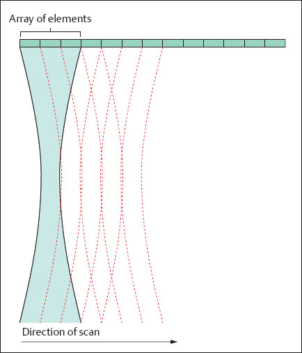
Fig. 1.14 Mode of operation of a modern ultrasound scanner.

Linear Array Scanner

Related posts:

Diagnosis of the Uterine Tube by Transvaginal Sonography Doppler Sonography in Obstetrics—Screening At-Risk Populations Doppler Ultrasound and the Cardiotocogram Indices for the Evaluation of Doppler Sonograms Doppler Ultrasound in the Diagnosis of Fetal Anomalies Vascular Supply of the Uteroplacentofetal Unit and Techniques for the Examination of Individual Vessels

Stay updated, free articles. Join our Telegram channel

Join