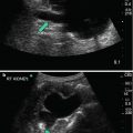
Principles and Applications of 3D Pelvic Floor Ultrasound

Fig. 9.1

(a, b) 3D volume acquisition. A series of sagittal (a) or axial (b) images are acquired by the transducer to obtain a 3D volume dataset

2D greyscale ultrasound imaging allows the operator to image the organ or region of interest in two planes (the sagittal and transverse planes). The ability to acquire a 3D ultrasound dataset (volume) allows reconstruction of the axial plane which is generally not able to be obtained in 2D imaging. This process is called multi-planar reconstruction, similar to the process of reconstructing images in sagittal and coronal planes on a CT scan.

The ability to perform volume rendering allows the user to reconstruct a 3D image which may help in diagnosis. There are also powerful algorithms that allow real-time updating of the 3D reconstructed image, producing a so-called ‘4D’ capability (the fourth dimension being time). These processes require considerable computing/post-processing of the echo information and together with the physical limits of ultrasound (e.g. Pulse repetition frequency, field of view, lines of sight, etc. – see Chap. 1) can lead to lower resolution of the reconstructed image.

Technique of 3D Volume Acquisition and Analysis

3D Definitions and instrumental controls:

Pixel – A term used to describe the basic unit of 2D information displayed on an ultrasound image. Each pixel is assigned a series of gray scale X and Y Values.
Voxel – A term used to describe the basic unit of 3D information, as it has an additional vector of Z attached to it, to specify its location in the 3D volume. It is assigned the same series of gray scale values X, Y and the additional Z.
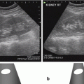
MPR (Multi planar reconstruction – Figs. 9.2 and 9.3) – MPR consists of the three planes that make up the 3D data set. They are positioned 90° from each other and labeled X, Y and Z. When one plane is manipulated, the other planes on view will change accordingly. Figure 9.4 illustrates the three MPR planes during 3D volume analysis. By convention the top left box is the acquisition plane, which is the sagittal plane in the example. This is the plane that was used initially to acquire the data set. The top right box is the orthogonal view to the acquisition plane. In the above case it’s the transverse view. The bottom left box is the coronal or C-plane view which is derived from the combination of acquisition and orthogonal views. This is the plane which is not generally possible on 2D imaging.

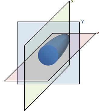
Fig. 9.2

Multiplanar reconstruction – the 3D ultrasound volume dataset can be analysed by manipulating the three planes (X, Y, Z) at right angles to each other

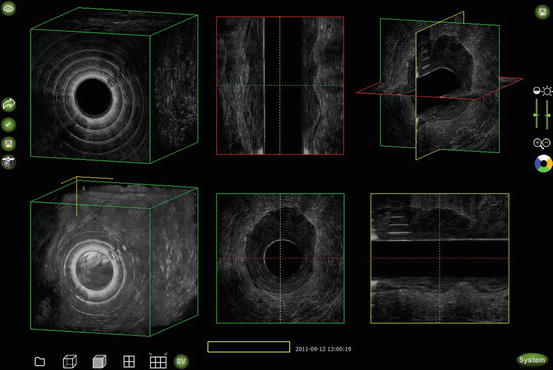
Fig. 9.3

MPR – 3D volume obtained by endoanal 3D transducer

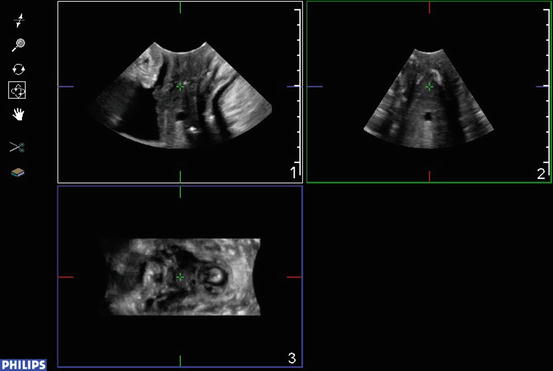
Fig. 9.4

Cross hair – this is a marker of the intersection of each plane. The intersecting point of the cross hair on each view represents the same point within the volume data set
Cross Hair – This is a marker of the intersection of each plane (Fig. 9.4). The intersecting point of the cross hair on each view represents the same point within the volume data set. Each plane rotates around the corresponding line that makes up the cross hair.
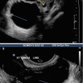
ROI – Region of Interest (Fig. 9.5). This is the user defined area on 2D imaging that is used to produce a 3D data set.

Fig. 9.5

Region of Interest (ROI). This is the user defined area on 2D imaging that is used to produce a 3D data set. The white triangular shaped area is the ROI box
Trim Line – In Fig. 9.5 the solid horizontal line is the trim line. Anything above this line will not be included in the 3D data set. Therefore, this line should be moved to the very top of the image so that information is not cut out of the data set.
Acquisition – This is the process of sweeping, pivoting or performing live 2D that will record a 3D volume.
Angle – This determines the range (thickness of the 3D volume) over which the acquisition will occur. Larger angle settings results in a larger volume acquired (Fig. 9.6).

Fig. 9.6

Sweep angle – this determines the range (thickness of the 3D volume) over which the acquisition will occur

Technique of 3D Data Acquisition (See Tips 9.1)

Obtain the best 2D image possible. In pelvic floor transperineal imaging this is achieved in the mid-sagittal plane. It is important to ensure there is adequate sonographic gel and enough pressure on the transducer to maintain good contact with the perineum and eliminate any air between the transducer and the perineum.

Initiate the 3D process.

Expand the ROI box (Fig. 9.5) to its maximum position to encompass the entire area of interest.

Increase the sweep angle (Fig. 9.6). If the region of interest is large (such as the pelvic floor) larger angles are required to capture the entire area.

Centre the ROI in the 2D image. For transperineal pelvic floor imaging it is helpful to use the urethra, vaginal canal or rectum as central landmarks. Obtain the best 2D image of the urethra, bladder, rectum, and vaginal canal as possible.

Activate the 3D sweep to capture the volume data.

Save the data set once this has been acquired making sure that it is the entire data set and not just the 3 plane-MPR image that is saved.

Reconstructing the Data Set

The easiest way to see if the data set is successful is to place the center of the cross-hairs in the center of the anatomical structure of interest (in the sagittal plane image). For example, place the cross hairs in the middle of the urethra, sling, mesh or anorectum. In the example dataset in Fig. 9.7, the suburethral sling will be used as the structure of interest. If the image is clearly defined in each of the three MPR views then a data set has been acquired that can successfully be manipulated.

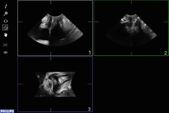
Fig. 9.7

A usable 3D volume dataset obtained by transperineal ultrasound of patient with mid-urethral sling – the image is clearly defined in each of the 3 MPR views

If the data set is usable then select the top left box for manipulation. Selecting an individual box on the MPR view allows manipulation of that particular view in all directions X, Y and Z. The top left box of the MPR data set is the acquisition plane. This is the plane used initially to acquire the data set. Manipulating the X, Y and Z planes will manipulate the view so that it is in the exact location to display the structures of interest. Manipulating the X plane while still in the acquisition plane will rotate the image like a rolodex (eg. elongate the urethra in this particular view to obtain a true sagittal section- Fig. 9.8).

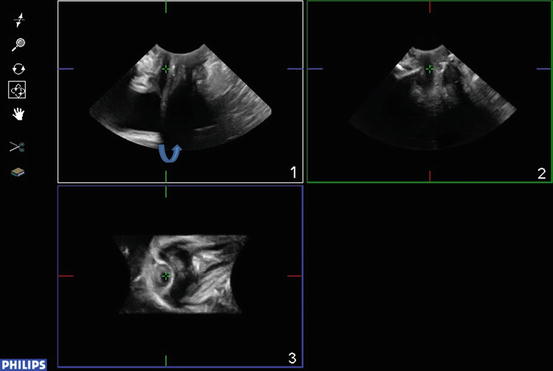
Fig. 9.8

MPR – manipulating the X plane. This will rotate the image like a rolodex (arrow), elongating the urethra in this particular view to obtain a true mid-sagittal section

Manipulating the Y plane will sweep the transverse image from the left arm of the sling to the right arm of the sling in the acquisition plane (like a revolving door) (Fig. 9.9). While manipulating the Z plane will cartwheel the image (Fig. 9.10).

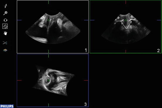
Fig. 9.9

MPR – manipulating the Y plane. This will sweep the transverse image from the left arm of the sling to the right arm of the sling (arrows) in the acquisition plane (like a revolving door)