Chapter 10 Principles and practice of radiation treatment planning
Introduction
The planner must take the clinical requirements stated in a prescription and planning request and translate them into the best plan for the individual patient. This must then be presented to the clinician in a clear format so that what in many cases is a complex three-dimensional plan can be readily appraised. Over the years, tools and techniques have evolved to enhance this critical communication between staff groups. The ICRU reports 50 and 62 [1, 2] referred to in Chapter 9 provide an effective methodology of prescribing the volume to be treated and the means of displaying the dose distribution produced by the treatment plan.
Table 10.1 gives typical tolerance doses for organs. However, these values should not be taken as absolute, as fractionation affects the ability of normal tissue to repair damage. The quoted dose may represent an increased risk rather than a stochastic threshold above which all patients will be affected. The patient’s clinical condition and drugs may affect radiosensitivity of some organs. The complete clinical picture is also important, for example in the abdomen region, the planner must know whether one of the kidneys is already non-functioning as this will enable them to design a plan that may reduce the dose to the healthy kidney at the expense of dose to the already damaged one.
Table 10.1 Typical normal tissue tolerance doses for generally accepted risks. Note that these may vary for individual situations due to clinical condition and other therapies increasing radiosensitivity and that correction must be made for different fractionation
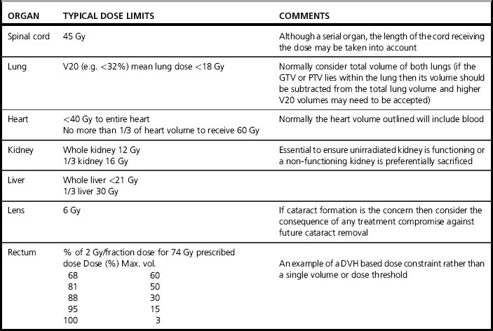
The reasoning behind the prescribed dose required to kill a specific tumour type is discussed in Chapter 17. The treatment planner is given this in the plan request and is solely concerned with delivering this dose at the specified fractionation. However, it is important to have the dose and dose per fraction available at the time of planning as the dose limits to critical structures will depend on the dose rate.
Patient data
The patient contours may be acquired in the form of multiple computed tomography (CT) slices or, in some cases, derived from external contours alone, possibly with some estimation of the dimensions and density of significant internal heterogeneities, such as the lung. The detailed anatomy derived from CT images is the optimum means of obtaining accurate dose distributions as the CT numbers can be converted to electron density maps, which the treatment planning computer (TPS) will use to calculate how the beams are attenuated and scattered. However, CT- density tables can also be manipulated to obtain enhanced digitally reconstructed radiographs (DRRs), so it is important to use a table that is specifically intended for dosimetry rather than imaging (see Chapter 9).
CT is the best imaging modality for radiotherapy in terms of dosimetry and spatial accuracy, but does not always provide the best images for tumour or critical structure localization. Normal practice is to register the diagnostically superior magnetic resonance (MR) or positron emission tomography (PET) images onto the CT images (see Chapter 9). However, it is possible to use the MR images directly for some sites, by applying distortion correction to the MR images and assigning ‘bulk heterogeneity’ corrections to visible structures such as bone.
Figure evolve 10.1 shows the effect of patient breathing on a thoracic CT image acquired in spiral mode. The appearance of the liver clearly indicates the breathing motion that otherwise might not be apparent.
Radiotherapy patients may have prostheses, dental fillings, breast implants, and other artifacts present externally or internally. Sometimes these will be present during imaging but may be removed by the time treatment commences (for example, drainage tubes). Where the artifact is made of material similar to tissue density such as breast implants (although some breast implants contain high-density magnets), the CT-density table will correctly allocate the density required. However, for metal implants, the CT scan must be acquired with an extended CT scale and the TPS CT-density table must be extended typically to give Hounsfield numbers of up to 32 000 if metal implants are to be identified and the correct density assigned. Even with artifact correction tools on CT scanners, there are usually significant artifacts present surrounding metal objects – especially for bilateral hip implants, and a manual overlay of the density may be required (Figure evolve 10.2 ). The use of MR imaging in the presence of non-ferrous implants may provide useful information that may be transferred to the distorted CT dataset.
Contrast may be present in a CT scan, for example, to visualize nodes in head and neck images (Figure evolve 10.3 ), or may be present in the bladder as a result of contrast used elsewhere.
Megavoltage photon therapy
Treatment beams
Beam energy
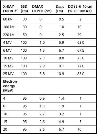
The first parameter the planner selects is the beam energy, by considering the depth of dmax and the penetration properties of the beam (Table 10.2 shows typical values for commonly used energies). Low energy beams, e.g. 4–6 MV are suited to more superficial volumes, e.g. head and neck PTVs, while deep pelvic PTVs will require 10–20 MV. Beam energies above 15 MV do not give a great benefit to the planner, but their frequent use on a Linac can introduce radiation protection problems from neutrons.
Wedges
Megavoltage treatment machines have integral beam modifying techniques which are referred to as wedges (see Chapter 8). They alter the uniform dose distribution of the radiation beam in a simple and controlled manner to produce a dose gradient across the field.
Wedges are essential for most multifield plans to produce a uniform PTV dose and serve two purposes.
First, they allow one field to compensate for the depth dose fall off of another field in the plan (Figure evolve 10.4A ). Secondly, they compensate for a ‘density gradient’ in the path of the beam (Figure evolve 10.4B, C
 ). The simplest application of this is ‘missing tissue’ when a beam enters an oblique patient contour, but heterogeneities within the patient may also require correction especially the lungs and large pelvic bones.
There are several techniques used in treatment machines for generating wedge-shaped isodoses (see Chapter 8) and the technology used can influence the plan. Fixed wedges may be positioned in the beam for the entire delivery of the beam. This is less commonly used as it requires each field to be manually set up inside the treatment room but, in some machines, may be the only method of permitting a wedge to be orientated in all four directions in the field. These are described in terms of wedge angle of the isodose distribution that they produce (not the physical shape of the wedge itself).
For the planner, there are a number of consequences arising from these different technologies.
The wedge direction may be limited, i.e. not both sets of jaws can generate dynamic wedges, or physical wedges cannot be rotated into both collimator planes. When planning with multileaf collimators, this may limit the effectiveness of the multileaf collimator (MLC) shielding if the wedge orientation restricts the planner to a suboptimal collimator rotation (Figure evolve 10.5 ).
).
Blocks
1. the penumbra is spread, more so the further the block is from the central axis
2. the limited range of block sizes may result in compromised shielding
Multileaf collimators (MLCs)
• the leaf width (defined at the isocentre) may be too coarse for effective collimation especially of small fields
• the orientation with respect to the wedge may not always provide the optimum shielding (see Figure evolve 10.5 )
)
• there may be unavoidable dose to normal tissue due to interleaf leakage, especially where a backup collimator is relied upon to minimize this effect (Figure evolve 10.6 ) but cannot be brought up to the field edge due to the shape of the PTV
• where MLCs replace both collimator pairs, one field dimension is limited to increments of the leaf width.
Planning tools, calculation and display
Algorithms for dose calculation in treatment planning systems
Algorithms can be represented as follows.
Stored beam data models
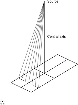
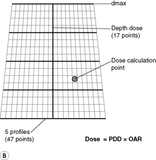
This algorithm is also frequently used as the method of point dose checking on an independent system. Measurements required are percentage depth doses (PDD’s) along the Central Axis (CAX) of the beam and off-axis ratios (OAR’s) in the form profiles across the beam (as shown in Figure 10.7A and B), output factors as a function of field size, wedge factors for each wedge, cGy/MU for reference situation with a 10 × 10 cm field and a knowledge of dmax depth. The planning computer can then interpolate these basic data and apply corrections to produce isodose curves in a tissue equivalent phantom. In order to calculate the dose to a patient, a heterogeneity correction is often applied. This can be done by various different methods, such as bulk density equivalent path length, pixel-by-pixel equivalent path length, power law method (Batho) or the ETAR method. Irregular fields are calculated using scatter integration techniques, such as the Clarkson method.
Pencil beam models
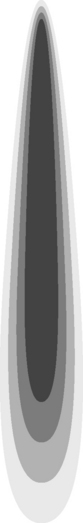
Pencil beam models have been introduced to provide a more accurate method of calculating irregular fields and are therefore more suitable for use in dosimetry of conformal radiotherapy and IMRT inverse planning algorithms. They are, however, still prone to some inaccuracy in very inhomogeneous situations. Figure 10.8 illustrates an example of a pencil beam kernel generated by a Monte Carlo calculation to represent the elemental dose distribution from a single infinitesimal beam element at a specific energy. Multiple elements are then summed to represent the total fluence across the radiation field as shown in Figure 10.9.
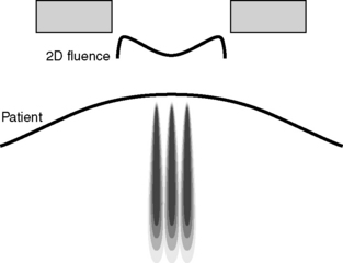
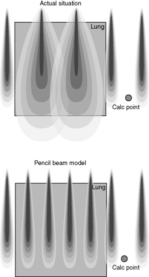
There are several limitations of this method in a clinical situation, such as in the calculation of dose to lung, as the side-scatter produced in a real situation is not correctly modelled as illustrated in Figure 10.10.
Treatment plan evaluation tools
Several such tools are in use as discussed.
Isodose distributions
Generally, isodose curves are normalized to give 100% to a reference point (such as the ICRU 62 reference point). This makes both the assessment of PTV coverage and the dose uniformity across the volume easier. The aim is usually to cover the PTV with the 95% isodose curve while ensuring the maximum dose within the volume does not exceed 107% [1, 2].
• opaque and translucent colour wash displays give a good overall impression of the dose distribution, but can obscure target volumes, so should be interchangeable with conventional isodose lines (Figure evolve 10.11 )
)
• isodose surfaces displayed as wire frames superimposed on rendered surfaces, with real time manipulation
• a ‘volume of regret’ is a dose reduction technique applied to the dose distribution. A window of acceptability of dose level is chosen and portions of organs outside this window can be highlighted. For critical organs, this is a one-sided test, where regions where the dose is above the acceptable level are displayed. For target volumes, regions of either too high or too low dose can be shown. This display feature is particularly useful when checking the coverage of arcing beams, e.g. for stereotactic radiotherapy.