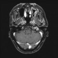
Radiobiological Principles Underlying Stereotactic Radiation Therapy

Fig. 5.1

Hypoxic regions (black) indicated by pimonidazole staining are present even in small tumors. Imaged here is a section of a small tumor derived from a human glioma xenograft line. Adapted from Rijken PF, Peters JP, Van der Kogel AJ. Quantitative analysis of varying profiles of hypoxia in relation to functional vessels in different human glioma xenograft lines. Radiat Res. 2002 Jun;157(6):626–32; used with permission

Figure 5.2 shows a dose–response curve, derived from the classic studies of Powers and Tolmach [30], illustrating the fraction of cells surviving in very small tumors in a mouse irradiated in a single fraction in vivo and subsequently assayed by transplantation to other animals. The cellular survival curve is characterized by two distinct components; the slopes of the two components differing by a factor of 2–3. Up to doses of several Gy, the response is dominated by the killing of aerobic cells, while, for higher doses, the killing of hypoxic cells dominates. It is apparent that irradiating such tumors with a single large dose of several tens of Gy is a futile exercise if the goal is sterilization, since the hypoxic cells will not be adequately depopulated with a dose of this magnitude. Figure 5.3 gives rough estimates [31], based on in vitro data, of the single fraction dose to sterilize a 30 mm diameter tumor, with and without a hypoxic component.

Fig. 5.2

Fraction of surviving cells, after a single radiation dose, in small mouse lymphosarcomas irradiated in vivo. The shallow initial part of the curve is due to the presence of aerated oxic cells, whereas the steeper slope at higher doses is caused by the presence of 1–2 % of hypoxic cells. Reprinted from Hall EJ, Brenner DJ. The radiobiology of radiosurgery: rationale for different treatment regimes for AVMs and malignancies. Int J Radiat Oncol Biol Phys 1993; 25:381–385. Copyright 1993, with permission from Elsevier

Fig. 5.3

Rough estimate, based on in vitro data, of the single-fraction dose required to sterilize various 30 mm diameter tumors, which are either fully oxygenated (lower) or contain 20 % hypoxic cells (upper). Adapted from Leith JT, Cook S, Chougule P, Calabresi P, Wahlberg L, Lindquist C, et al. Intrinsic and extrinsic characteristics of human tumors relevant to radiosurgery: comparative cellular radiosensitivity and hypoxic percentages. Acta Neurochir Suppl. 1994;62:18–27; used with permission from Springer Science + Business Media

However, malignant tumors exhibit a characteristic known as reoxygenation whereby, between fractionated doses of x- or γ-rays, tumors tend to reestablish their original pattern and proportion of oxygenated and hypoxic cells. This principle is illustrated in Fig. 5.4 [32]. In a fractionated regime, therefore, each X- or γ-ray dose predominantly kills aerobic cells, and the interval between treatments allows hypoxic cells to reestablish their oxygenated state, thereby reducing the problem of hypoxic radioresistance. An analysis [33] of survival data for cervix cancer patients undergoing fractionated external-beam radiotherapy and high dose-rate brachytherapy suggests the clinically relevant oxygen enhancement ratio (OER) for hypoxic tumor subvolumes may be closer to 1.5, substantially lower than the typically reported value of ~3 for in vitro clonogenic survival under anoxic conditions. An OER of 1.5 agrees with values reported in vitro for oxygen concentrations of ~5 mmHg (0.66 %). However, clinically derived OER values are averaged over cells under a range of oxygen concentrations, so cells irradiated in vivo under extreme levels of hypoxia, e.g., <0.5 mmHg, may still have OER values higher than 1.5.

Fig. 5.4

Schematic illustration of the process of reoxygenation: almost all tumors initially contain a mixture of aerated and hypoxic cells. A single radiation dose will kill a larger fraction of aerated oxic cells because they are more radiosensitive (see Fig. 5.2). Thus after irradiation, a larger fraction of cells are hypoxic. But after a short time, the tumor tends to return to its original proportion of oxic and hypoxic cells, allowing many of the previously hypoxic (but now aerated) cells to be killed by a second, and subsequent, dose fractions. Reprinted from Hall EJ, Brenner DJ. The radiobiology of radiosurgery: rationale for different treatment regimes for AVMs and malignancies. Int J Radiat Oncol Biol Phys 1993; 25:381–385. Copyright 1993, with permission from Elsevier

While stereotactic techniques offer valuable physical advantages over conventional radiotherapy, the potential for reoxygenation is reduced as the total dose is delivered in a fewer number of fractions. Hypofractionation may result in decreased biological effectiveness for hypoxic tumors [34]. The clinical significance of tumor hypoxia and reoxygenation within the context of SRT is still a subject of rigorous debate [35].

Repair

The second radiobiological principle is repair of DNA damage. It has been well established for many decades that protracting or fractionating an acute exposure reduces the level of cell killing. An example is shown in Fig. 5.5. If all tissues were equally affected by changes in protraction or fractionation, then there would be no radiotherapeutic significance to fractionation, beyond the need to increase the dose to compensate for the increased cellular repair of double-strand breaks (DSBs).

Fig. 5.5

Illustrating that, as a given single dose is protracted, either by lowering the dose rate (as here) or by increasing the number of fractions, the biological effect (in this case, cell killing of Chinese hamster cells) decreases, due to intra-fraction double-strand break (DSB) repair. Based on data from Bedford JS, Mitchell JB. Dose-rate effects in synchronous mammalian cells in culture. Radiat Res. 1973 May;54(2):316–27. Reprinted from Hall EJ, Brenner DJ. The dose-rate effect revisited: radiobiological considerations of importance in radiotherapy. Int J Radiat Oncol Biol Phys 1991; 21:1403–1414. Copyright 1991; with permission from Elsevier

However, there is a wealth of experimental evidence which indicates that there is a difference in shape between the dose–response relationship characteristic of early responding tissues and tumors and late responding tissues. The inference from experiments in animals, which is confirmed in clinical practice, is that the dose–response relationship for late responding tissues has more curvature than that for early responding tissues, as shown in Fig. 5.6.

Fig. 5.6

The gamma ray dose–response curve for late responding tissues (e.g., AVM obliteration, cerebral necrosis) has more curvature, i.e., a small α/β ratio; for early responding endpoints such as tumor control, the dose–response curve is straighter, i.e., the α/β ratio is larger. Consequently dose fractionation spares late responding tissues more than early responding tissues. Reprinted from Hall EJ, Brenner DJ. The radiobiology of radiosurgery: rationale for different treatment regimes for AVMs and malignancies. Int J Radiat Oncol Biol Phys 1993; 25:381–385. Copyright 1993, with permission from Elsevier

In mathematical terms, if the dose (D)–survival (S) relationship is expressed in terms of a linear–quadratic relation,

$S= \exp \left(-\alpha D-\beta {D}^2\right),$

(5.1)

then the ratio α/β (the dose at which the cell killing by the linear and quadratic terms is equal) tends to be small for late responding tissues (less than ~3 Gy) and larger (greater than ~8 Gy) for early responding tissues [32, 36–40].

The practical consequence of the difference in shape between the dose–response curves for early and late responding tissues is a marked difference in the response to fractionation of these two types of tissues. Late-responding tissues are more sensitive to changes in fractionation than early responding tissues. The overall outcome is illustrated in Fig. 5.6. A fractionated regime spares late responding normal tissues more than a single acute dose, for a given level of tumor damage.

It is pertinent to ask what exactly constitute “early” and “late” responding tissues. Probably early responding tissues contain a large proportion of cycling cells, while late responding tissues contain large proportions of non-cycling cells.

Accelerated Repopulation

As a tumor shrinks during radiotherapy, the surviving clonogens are stimulated to proliferate at an accelerated rate [41, 42]. For T₃ laryngeal cancer, this accelerated repopulation does not commence for about 30 days after the beginning of treatment as illustrated in Fig 5.7 [43]. Radiation treatments of duration longer than about 30 days would therefore need to increase the total dose to compensate for this clonogen proliferation. Note that it is unrealistic to categorize almost any tumor type as one which is not significantly prone to repopulation—if research in predictive assays has taught us anything, it is that inter-tumor variation can be large; thus, in this context, some tumors will grow slowly and some will grow very quickly. For example, it has been suggested that the onset to repopulation may be as long as 60 days for slowly proliferating prostate tumors [44].

Fig. 5.7

Tumor control probability for T3 laryngeal cancer, as a function of overall time and overall dose. The data points, at the top of the dashed vertical lines, are those reported by Slevin et al. [43], and the surface is the result of a linear–quadratic (with repopulation) fit [42] to the data, with repopulation effectively starting about 33 days after the beginning of the treatment. Reprinted from Brenner DJ. Accelerated repopulation during radiotherapy: quantitative evidence for delayed onset. Radiat Oncol Invest 1993; 1:167–172. Used with permission

How Do These Radiotherapeutic Principles Apply to Stereotactic Radiation Therapy?

In general these three phenomena control the dose delivery for cancer radiotherapy as follows:

We must fractionate treatment:

To overcome hypoxia
For differential response with late effects

We would like to prolong treatment:

To limit early sequelae

We would like to shorten treatment:

To prevent accelerated repopulation

Prima facie, requirements 2 and 3 are mutually exclusive and so, in most radiotherapeutic situations, the overall treatment time represents a compromise between short treatment times to minimize tumor repopulation and long treatment times to prevent unacceptable early complications. In those protocols that have attempted to utilize shorter overall treatment times, it has been necessary to reduce the overall dose in order to avoid excessive early complications [45].

By contrast, stereotactic radiotherapy represents a situation where the contradictory aspects of overall treatment time can be resolved without the need for compromise. Because of the excellent dose distributions which can be obtained using stereotactic radiotherapy, the need for long overall treatment times to reduce early normal tissue complications will rarely apply. Specifically, early skin or mucosal reactions, which are often a limiting factor in radiotherapy, will not be an issue for intra-cranial stereotactic radiotherapy. Thus short overall treatment times become a practical possibility, with their attendant advantages in terms of limiting tumor repopulation.

Inherently, then, SRT is advantageous in terms of repopulation. We discuss here how the remaining two Rs of radiotherapy (reoxygenation and repair) affect stereotactic radiotherapy for the three main target lesions, malignancies, AVMs, and benign tumors.

Malignancies

As we have discussed, it is very unlikely that a single dose fraction could sterilize even a small tumor which contains hypoxic malignant cells. Thus there is a clear rationale, based on the issue of hypoxia, for stating unequivocally that single-fraction radiotherapy, radiosurgery, is a suboptimal modality when the target is a malignant tumor [46].

In addition, because of the differential α/β ratio of the tumor and the surrounding late responding normal tissue sequelae (such as delayed cerebral necrosis, or optic neuropathy), even in the rare situation when there is minimal hypoxia, single-fraction treatment of a malignancy would be expected to give a suboptimal therapeutic ratio between tumor control and late complications.

Thus an optimal stereotactic radiotherapy protocol for a large intra-cranial malignancy would involve large numbers of fractions over a short time period, for example, 20 fractions in 2 weeks might be an appropriate target. For smaller tumors, where the relative dose to normal tissue surrounding the malignancy is smaller—though still, as always, dose limiting—a regime consisting of five or ten fractions over 1 week would combine the clinical advantages of a very short overall time, the radiobiological advantages of reoxygenation and (partial) repair of late responding normal tissue damage, and the practical advantages of a small number of treatments.

It has been argued [47] that, even for malignancies, “when the treatment volume is small and contains little functioning brain tissue, the need for fractionation may not apply.” However, the dose-limiting factor of any radiotherapeutic treatment of a malignancy must always be the normal tissue tolerance, so fractionation should always allow a greater tumoricidal dose.

Of course one of the potential advantages of radiosurgery is that it may be able to overcome the radioresistance of tumors such as metastases from melanomas or renal-cell sarcomas. However, by keeping the number of fractions low (perhaps to five or six), the radioresistance of such tumors will still be adequately addressed while maintaining the other biological advantages of fractionation that have been outlined here.

The arguments presented here do not exclude the fact that good results may be obtained using radiosurgery for brain malignancies. Indeed there are reports of good results with this technique. Rather, for any given situation, better results—in terms of therapeutic ratio between tumor control and complications—would always be expected by fractionating than can be obtained with a single fraction—an important consideration in the treatment of cerebral malignancies.

Arteriovenous Malformations

In treating AVMs, the goal is to produce progressive luminal closure through an inflammatory reaction in the vessel walls of the malformation, by irradiating the constituent epithelial cells [48–51]. This is a classic “late” response, occurring weeks to months after the radiation treatment and thus, prima facie, one would expect a relevant α/β ratio similar to that for other late responding tissue.

The issue here is that the dose-limiting side effect of the treatment, generally delayed cerebral radionecrosis, is, of course, also a late response [52–56]. Thus, in the treatment of AVMs, the tissue which it is desired to damage and the surrounding normal tissue that it is desired to spare are both of the same radiobiological type, i.e., they are both late responding tissues. Consequently one would expect that nothing is to be gained by a fractionated course relative to a single dose. In other words a change in fractionation pattern will not preferentially produce more damage in the AVM than in the surrounding normal tissues. The ratio of damage between the AVM and the surrounding normal tissue would be the same whether the dose is delivered in a single or in multiple exposures. Given that the issue of hypoxic cells is not relevant here, this is a strong rationale for radiosurgery, i.e., a single, highly localized radiation treatment.

In fact, there have been few estimates of α/β ratios reported in the literature corresponding to the end point of AVM obliteration, as few dose–response data have been established. An early estimate [46] of 0.6 Gy (range 0.2–5 Gy) was reported based on limited dose–response results for complete AVM obliteration after stereotactic irradiation with helium ions. Using the more recent dose–response data from Touboul et al. [57] and Flickinger [58], we estimated values of 5.2 Gy from long-term obliteration data and 2.4 Gy [range 0.9–8 Gy] from short-term obliteration data (see Fig. 5.8). A recent analysis by Kocher et al. [59] of most available data resulted in an overall best estimate of 3.5 Gy and an estimate of 4.6–6.4 Gy for small AVMs. All these values are consistent with those of a classic late response.

Fig. 5.8

Linear–quadratic fit to combined long-term AVM obliteration data from Paris [57] and Pittsburgh [58]. The estimated α/β ratio from this analysis is 5.2 Gy, consistent with a recent estimate of 3.5 Gy by Kocher et al. [59], based on most currently available data, which is in turn consistent with a typical α/β value for a late responding tissue

In summary, in the treatment of AVMs there is probably nothing to be gained by a fractionated course relative to a single dose. Thus, the optimal treatment for AVMs is expected to be single-fraction stereotactic radiotherapy or radiosurgery, i.e., a single, highly localized radiation treatment at, of course, the appropriate dose.

Benign Tumors

Less is known about the sensitivity to fractionation of benign tumors. It is less likely that hypoxia will be a significant role here [60]; one estimate of the α/β ratio for benign parasellar meningiomas is 3.3 Gy [61], similar to that for late responding normal tissues. For benign tumors as with AVMs, the most likely scenario is that both the target and the surrounding normal tissue respond in a similar way to fractionation, like that of a late responding normal tissue, suggesting that there is little to be gained from fractionation. For example, if the dose-limiting late sequelae were radiation-induced optic neuropathy, which is caused by damage to the arteries supplying the optic nerve, this almost certainly responds to changes in fractionation like a classic late responding tissue [62, 63].

In summary, in the treatment of benign tumors there is probably nothing to be gained by a fractionated course, relative to a single dose. However, we certainly do not have adequate data for a variety of benign tumors to consider this conclusion definitive.

Mechanistic Models of Radiotherapeutic Response

Why are we interested in mechanistic models to describe radiotherapeutic response? There are really two reasons: First, we need some model for calculating isoeffect doses when alternate fractionation schemes are considered. Second, mechanistic models are a useful tool for understanding mechanisms—if a model based on given mechanisms is inconsistent with the data, then we can conclude that the assumed mechanism is either wrong or not the dominant one.

The tool most commonly used for quantitative predictions of dose and fractionation dependencies is the linear–quadratic (LQ) formalism [37, 38, 64–66]. In radiotherapeutic applications, the LQ formalism is now almost universally used for calculating isoeffect doses for different fractionation/protraction schemes.

In contrast to earlier methodologies, such as CRE, NSD, and TDF [67, 68], which were essentially empirical descriptions of past clinical data, the LQ formalism has become the preferred tool largely because it has a somewhat more biological basis, with tumor control and normal tissue complications specifically attributed to cell killing. By contrast, descriptive empirical models can go disastrously wrong if used outside the dose/fractionation range from which they were derived—as when NSD was applied to large doses per fraction [69, 70].

Mechanistic Basis of the Linear–Quadratic Model

The standard model is that both tumor control and complications result primarily from cell killing [38, 71, 72]—and the LQ is a mechanistic model of cell killing (though see below for discussions of possible alternate mechanisms). In Eq. (5.1), αD can be interpreted as the quantity of lethal DNA lesions formed by a single radiation track, i.e., unrejoinable DSBs, lethally misrepaired or fixed DSBs, and lethal intra-track exchange-type chromosome aberrations, while βD2 can be interpreted as the quantity of lethal DNA lesions formed by two radiation tracks, i.e., lethal inter-track exchange-type chromosome aberrations formed through binary misrepair of two separate DSBs [66, 73]. Underlying the application of the LQ to fractionation and protraction effects is the pairwise misrepair of primary lesions such as DSBs or base damage formed by separate radiation tracks (hereon in, we shall refer to the DSB as the primary lesion, but base damage sites may well also be relevant here [74]). As schematized in Fig. 5.9, cell killing can occur via chromosome aberrations such as dicentric aberrations [75], formed when pairs of nearby DSBs wrongly rejoin to one another [76]. Protracting the exposure time potentially allows the first DSB to be repaired before the second is produced, and the LQ approach quantifies this effect [66]. Nowadays, this binary DSB misrepair model is the most usual way to motivate the standard LQ approach, but different biological rationales for the same mathematical formalism have also been given, as we will discuss.

Fig. 5.9

Examples of binary misrepair: (a) shows two chromosomes; each has one double strand break (DSB), shown as a gap. Centromeres, which are needed for proper transmission of chromosomes to daughter cells at mitosis, are shown as black constrictions. Most DSB are correctly restituted, but a few undergo binary misrepair. (b) Binary misrepair can result in a dicentric chromosome aberration, which generally destroys the clonogenic viability of the cell. In about half the binary misrepair events, the two DSBs shown in (a) lead to a translocation (c). Translocations involve large scale rearrangements and can cause potentially precarcinogenic alterations in cellular phenotype but most do not impair cellular survival. Reprinted from Brenner DJ. The linear–quadratic model is an appropriate methodology for determining isoeffective doses at large doses per fraction. Semin Radiat Oncol. 2008; 18: 234-239. Used with permission

It is important to stress here that the standard LQ formalism, as applied to time–dose relationships, is not merely a truncated power series in dose. Its key feature here is a specific mechanistically based functional form for the protraction factor, usually designated by G, which takes into account dose protraction or fractionation. Expressions for special cases of the time factor, G, were derived by Lea and Catcheside [65, 77]; a general form was subsequently derived [78] and has since been rederived from several different points of view [70]. We refer to this general form of the time factor, given explicitly in Eq. (5.5), as the generalized Lea–Catcheside time factor, G.

The LQ Formalism

The LQ model, in its most usual current version, describes cell killing in terms of the following mechanisms:

Radiation produces many types of clustered DNA lesions, including the DSBs, proportional to absorbed dose up to several hundred Gy for low- and high-LET radiation [79–82]. Experiments such as these imply that single-track mechanisms are responsible for the induction of DSBs and all other types of clustered DNA damage.

These DSBs can be repaired, with first-order rate constant λ(=ln 2/T _½, where T _½ is the repair halftime). In practice, there may be more than one class of DSB which may be repaired with different rate constants; the LQ formalism can be simply extended to take this into account.

In competition with DSB repair, binary misrepair of pairs of DSBs produced from different radiation tracks (i.e., different photons) can produce lethal lesions (often identified as predominantly dicentric chromosomal aberrations), the yield being proportional to the square of the dose (see the quadratic term in Eqs. 5.2 and 5.4). The two independent radiation tracks can occur at different times during the overall regimen, allowing repair of the first DSB to take place before it can undergo pairwise misrepair with the second; it is this phenomenon which is the heart of the fractionation/protraction dependence in the LQ formalism.

In addition, single radiation tracks can produce lethal lesions, possibly by a variety of mechanisms, the yield being linearly proportional to the dose.

Overall, in the LQ formalism, the yield (Y) of lethal lesions and the corresponding survival (S) equation are

$Y\propto \alpha D+G\beta {D}^2.$

(5.2)

(Note that the biologically effective dose, biological effective dose (BED), is defined as Y/α [37].) Then, assuming the lethal lesions are Poisson distributed from cell to cell, the surviving fraction will be

$S= \exp \left(-Y\right),$

(5.3)

and thus

$S= \exp \left[-\left(\alpha D+G\beta {D}^2\right)\right].$

(5.4)

In Eqs. (5.2) and (5.4), G is the generalized Lea–Catcheside time factor, which accounts quantitatively for fractionation/protraction; it is important to note that G acts only on the quadratic component, as described in Point 3 above. The generalized time factor has the form [78]

$G=\left(2/{D}^2\right)\underset{-\infty }{\overset{\infty }{{\displaystyle \int }}}\dot{D}(t)dt\underset{-\infty }{\overset{t}{{\displaystyle \int }}}{e}^{-\lambda \left(t-{t}^{\prime}\right)}\dot{D}\left({t}^{\prime}\right)d{t}^{\prime }.$

(5.5)

Here $\dot{D}(t)$ describes the variation in dose rate over the entire course of the radiotherapy, and λ is a characteristic damage repair rate. Generically, the term after the second integral sign refers to the first of a pair of DSBs required to produce a lethal lesion—the exponential term describing the reduction in numbers of such DSB through repair; similarly, the term after the first integral sign refers to the second DSB, which can interact with DSBs, produced earlier, that still remain after repair.

The time factor, G, can be calculated for any fractionation/protraction scheme and systematically accounts for the effects of protracting the dose delivery in any way. G can take values from zero to one, with G = 1 for a single acute dose, leading to the simplest single-fraction LQ formalism shown in Eq. (5.1). The interpretation of G < 1 is a reduction in cell killing due to intra-fraction DNA repair which occurs during protracted radiotherapy. Two special cases, which illustrate the main features of the general expression for G, are: (1) for irradiation with n short fractions, each separated by a time T [83]:

$G=\left[2\theta /\left(1-\theta \right)\right]\left[n-\left(1-{\theta}^n\right)/\left(1-\theta \right)\right],$

(5.6)

where θ = exp(−λ T). When the time between the short fractions is very long, then

(5.7)

and the most simple LQ model for well-separated fractionated exposures becomes

$S= \exp \left[-D\left(\alpha +\beta D/n\right)\right].$

(5.8)

Different fractionation/protraction schemes have different time factors, G, any of which can be calculated [64, 84] from Eq. (5.5). Even for high dose rates, dose protraction effects may have a significant impact on cell killing and, ultimately, treatment effectiveness [85, 86].

The LQ model can further be used to relate cell death to clinical endpoints of interest. The tumor control probability (TCP) model quantifies the response of a group of patients to a specific radiotherapy treatment and is essential in the analysis of clinical data for local control. The TCP model relates the tumor volume (or number of tumor cells) and the radiation dose to the probability of tumor cure, i.e., the probability that no tumor cells survive the radiation treatment. The most commonly used TCP algorithm [87, 88] is based on Poisson statistics:

$\mathrm{T}\mathrm{C}\mathrm{P}= \exp \left[-N\cdot S(D)\cdot {e}^{\gamma \left(T-{T}_{\mathrm{k}}\right)}\right],$

(5.9)

where N is the initial number of tumor clonogens, S(D) is the surviving fraction of cells predicted by the LQ model, T is the overall treatment time, and T _k is the lag time before accelerated tumor repopulation begins. The repopulation rate of tumor cells, γ, is conveniently expressed as γ = ln(2)/T _d, where T _d is the effective tumor doubling time. The TCP formalism can also be modified to include interpatient variability in radiosensitivity [89].

How Well Does the LQ Model Work, At Low and High Doses?

The goal here is to be able to make equi-effect regimen extrapolations from standard regimes, typically with 1.8–2 Gy per fraction, to hypofractionated regimes. Possible hypofractionated doses per fraction are, for example, up to about 7 Gy for prostate [90], and up to about 15–20 Gy for non-small cell lung cancer (NSCLC) [91]. For fractionated stereotactic radiotherapy, we are interested in extrapolating in the opposite direction, from single-fraction doses as high as 18 Gy to hypofractionated exposures with lower doses per fraction [92].

So the general question is whether the LQ formalism described in the previous section describes radiotherapeutically relevant dose–responses in the dose-per-fraction range from, say, 1.8 to 20 Gy. For many situations, such as prostate cancer hypofractionation, the dose-per-fraction range of interest is probably about 1.8–7 Gy.

Only gold members can continue reading. Log In or Register to continue