the field of real numbers, and with  Euclidean plane, the elements of which are vectors:
  means that
  , where both x and y are real. For any two vectors a and b from
  , their scalar product is defined by
  . With
  , we denote the unit vector
  . The distribution of the specific parameter within the slice through the body is described by the object function
  supported on the disk
  . It is supposed that
  , which means that
  . The Fourier transform of
  is defined by

(6.1)
From the fact that the object function  is finitely supported, it follows that its Fourier transform is infinitely supported. Therefore, its inverse Fourier is expressed by

where the integration is carried out over the whole plane  . The Radon transform of the function
  can be defined by

where  is the line described by parameters
  . The type of these parameters defines the type of the parameterization of the Radon transform. Commonly used is a
  -parameterization:

 is finitely supported, it follows that its Fourier transform is infinitely supported. Therefore, its inverse Fourier is expressed by
(6.2)
 . The Radon transform of the function
  can be defined by
(6.3)
 is the line described by parameters
  . The type of these parameters defines the type of the parameterization of the Radon transform. Commonly used is a
  -parameterization:
(6.4)
If parameter  is fixed, then
  generates a family of parallel lines. According to this, the parallel Radon projection in the direction
  is defined as

 is fixed, then
  generates a family of parallel lines. According to this, the parallel Radon projection in the direction
  is defined as
(6.5)
Depending on the situation, different notations, the sense of which will be always clear from the context, will be used, e.g.,  ,
,  , or
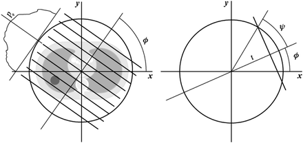
, or  . If alternatively instead of t the angle parameter ψ is used (see Fig. 6.1, right), we speak of
  parameterization. The line within this parameterization is expressed by

 ,
,  , or
, or  . If alternatively instead of t the angle parameter ψ is used (see Fig. 6.1, right), we speak of
  parameterization. The line within this parameterization is expressed by
(6.6)
Let  be coordinates in the coordinate system that is rotated relative to
  at angle
  :
:

 be coordinates in the coordinate system that is rotated relative to
  at angle
  :
:
(6.7)
We speak of  and
and  parameterizations of the Radon transform if

and

respectively. Families  and
and  where only
  is fixed generate fans of rays with an apex lying on the boundary of the disk
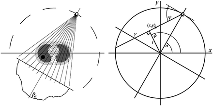
  . Therefore, both (6.8) and (6.9) are appropriate for the description of data collected over rays emitted by a point source moving along the boundary of the disk (Fig. 6.2).
 and
and  parameterizations of the Radon transform if
(6.8)

(6.9)
 and
and  where only
  is fixed generate fans of rays with an apex lying on the boundary of the disk
  . Therefore, both (6.8) and (6.9) are appropriate for the description of data collected over rays emitted by a point source moving along the boundary of the disk (Fig. 6.2).
Fig. 6.2
Fan-beam projection (left); setup for fan-beam geometry (right)
One of the important problems in practical tomography is the identification of optimal sampling conditions that must be imposed on the Radon transform. Because of limitations of the data acquisition system of the scanner, only discretized approximation of the Radon transform can be obtained. Therefore, on the one side, it is important to know how many data have to be collected in order to fully exhaust the potential of the scanner. On the other side, the radiation dose must be as small as possible, and therefore, the sparsest sampling scheme has to be identified among all of those which ensure the best approximation of the Radon transform. In connection to this problem, the Radon transform is supposed to be sampled on the lattice  , the elements of which are discrete points of the plane
  coordinated by parameters of the Radon transform (e.g., parameters
  ). So-called admissible lattice can be generated by a
  matrix
  such that
  , i.e., for any
  ,
,

 , the elements of which are discrete points of the plane
  coordinated by parameters of the Radon transform (e.g., parameters
  ). So-called admissible lattice can be generated by a
  matrix
  such that
  , i.e., for any
  ,
,
(6.10)
Lattice  is called dual or reciprocal to the lattice
  if for any
  andany
 , the scalar product
  . The generator matrix of the reciprocal lattice is

where the superscript  means transposition (see, e.g., [2]). Let the power spectrum of a function g be supported on the compact region
  . The fundamental result of the sampling theory is as follows: if regions
  and
and  are disjoint for any
  , then
  , where
  is the inverse Fourier transform of the function
  ,
,  if
if  , and otherwise
  (see [3]). In other words, the band-limited function can be exactly recovered from its discrete samples if the sampling conditions stated above are satisfied. From the definition of the reciprocal lattice, it follows that the denser
  is, the sparser is
  and vice versa. Therefore, if we want the sampling lattice
  to be as sparse as possible, we have to find such a reciprocal lattice
  that allows us to pack R2 with mutually disjoint replicas of the
  -region as tightly as possible. Certainly, the crucial role in doing this plays the shape of the
  -region.
 is called dual or reciprocal to the lattice
  if for any
  andany
 , the scalar product
  . The generator matrix of the reciprocal lattice is
(6.11)
 means transposition (see, e.g., [2]). Let the power spectrum of a function g be supported on the compact region
  . The fundamental result of the sampling theory is as follows: if regions
  and
and  are disjoint for any
  , then
  , where
  is the inverse Fourier transform of the function
  ,
,  if
if  , and otherwise
  (see [3]). In other words, the band-limited function can be exactly recovered from its discrete samples if the sampling conditions stated above are satisfied. From the definition of the reciprocal lattice, it follows that the denser
  is, the sparser is
  and vice versa. Therefore, if we want the sampling lattice
  to be as sparse as possible, we have to find such a reciprocal lattice
  that allows us to pack R2 with mutually disjoint replicas of the
  -region as tightly as possible. Certainly, the crucial role in doing this plays the shape of the
  -region.
In some parts of the text, concepts from the theory of distributions (see, e.g., [4, 5]) are used. Within the framework of this theory, one defines the set  of test functions. The distribution f over this set is to be understood as a map
  defined as follows: for
  ,
,
![$$ f[h]=\left\langle {f,h} \right\rangle =\int {f(x)\overline{h(x)}\mathrm{ d}x}. $$](/wp-content/uploads/2016/08/A270527_1_En_6_Chapter_Equ000612.gif)
 of test functions. The distribution f over this set is to be understood as a map
  defined as follows: for
  ,
,![$$ f[h]=\left\langle {f,h} \right\rangle =\int {f(x)\overline{h(x)}\mathrm{ d}x}. $$](/wp-content/uploads/2016/08/A270527_1_En_6_Chapter_Equ000612.gif)
(6.12)
In the imaging science, such an approach is justified, e.g., when the output of the imaging system can be described in terms of the convolution with the impulse response  . Let the function
  be smooth, symmetric, and compactly supported, and let its Fourier transform
  be essentially supported1 on the interval
 ![$$ [-w,w] $$](/wp-content/uploads/2016/08/A270527_1_En_6_Chapter_IEq000675.gif) . Beyond this interval,
. Beyond this interval,  is required to decay faster than any degree of
  . We define the set
  as a family
  of translates of the impulse response e, i.e.,
  . The set of Fourier transforms of test functions is
  , where

 . Let the function
  be smooth, symmetric, and compactly supported, and let its Fourier transform
  be essentially supported1 on the interval
 ![$$ [-w,w] $$](/wp-content/uploads/2016/08/A270527_1_En_6_Chapter_IEq000675.gif) . Beyond this interval,
. Beyond this interval,  is required to decay faster than any degree of
  . We define the set
  as a family
  of translates of the impulse response e, i.e.,
  . The set of Fourier transforms of test functions is
  , where
(6.13)
Then the Fourier transform of the distribution is defined as a map  such that
  for any
  .
.
 such that
  for any
  .
.6.3 Convolution-Based Algorithms
6.3.1 Parallel-Beam Geometry
The  parameterization is the most clear among all useful parameterizations of the Radon transform mentioned above. Being intensively investigated on the eve of practical tomography, the inversion of the Radon data collected within the parallel-beam geometry is fully understood today. Some important notions, such as, e.g., the resolution of the reconstruction, have been introduced and described for this kind of data geometry. Also the practical fan-beam inversion formulae are the result of the re-parameterization of the inversion formula obtained for the parallel-beam geometry.
 parameterization is the most clear among all useful parameterizations of the Radon transform mentioned above. Being intensively investigated on the eve of practical tomography, the inversion of the Radon data collected within the parallel-beam geometry is fully understood today. Some important notions, such as, e.g., the resolution of the reconstruction, have been introduced and described for this kind of data geometry. Also the practical fan-beam inversion formulae are the result of the re-parameterization of the inversion formula obtained for the parallel-beam geometry.
Let  be the Radon projection of the object function
  measured at angle
  . Due to (6.5), its 1D Fourier transform with respect to t is

 be the Radon projection of the object function
  measured at angle
  . Due to (6.5), its 1D Fourier transform with respect to t is
(6.14)
The identity (6.15) is the statement of the so-called Fourier slice theorem. By taking the inverse Fourier transform, this identity can be rearranged to

(see [6] for details). The formula (6.16) makes little sense if the product  is not absolutely integrable, what can be, e.g., in the case if
  . In order to stabilize it, let us multiply both sides of (6.15) with the term
  and handle the resulting identity in terms of distributions over the set B defined above. That is,

or, written in explicit form,


(6.16)
 is not absolutely integrable, what can be, e.g., in the case if
  . In order to stabilize it, let us multiply both sides of (6.15) with the term
  and handle the resulting identity in terms of distributions over the set B defined above. That is,
(6.17)

(6.18)
Setting  , integrating over
  from
from  to
to  , rearranging the right-hand side appropriately, and changing the variables from polar to rectangular in the double integral on the right-hand side of (6.18) yield

 , integrating over
  from
from  to
to  , rearranging the right-hand side appropriately, and changing the variables from polar to rectangular in the double integral on the right-hand side of (6.18) yield
(6.19)
The right integral in (6.19) is the inverse Fourier transform (up to the term  ) of the 2D convolution
  , where
  is a radial function such that
  . Hence, we obtain the inversion formula

which has the same structure as (6.16), but


 ) of the 2D convolution
  , where
  is a radial function such that
  . Hence, we obtain the inversion formula
(6.20)

(6.21)

(6.22)
Owing to the conditions imposed on  (see (6.13) and related discussion in Sect. 6.1), the formula (6.20) makes sense for any object function. Clearly, in terms of convolution, the formula (6.20) takes a form given by

where  is the parameter of the ray that goes through the point
  and
and

 (see (6.13) and related discussion in Sect. 6.1), the formula (6.20) makes sense for any object function. Clearly, in terms of convolution, the formula (6.20) takes a form given by
(6.23)
 is the parameter of the ray that goes through the point
  and
and
(6.24)
The formula (6.23) is called filtered back projection (FBP) because the evaluation of  can be accomplished in two steps: the convolution of Radon projections with the kernel
  (filtering) and evaluating
  with averages of
  (back projection).
 can be accomplished in two steps: the convolution of Radon projections with the kernel
  (filtering) and evaluating
  with averages of
  (back projection).
Note that (6.22), where on the right there is a convolution of parallel Radon projections with the impulse response of the imaging system, can be thought of as a model of measuring process. It is easy to check that

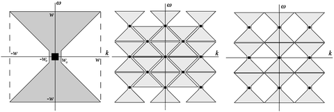
that is, the data obtained with the acquisition system of scanner are equivalent to Radon transform of the band-limited function F defined by (6.21). In [7], it was shown that the Fourier transform of the Radon transform of a band-limited function is essentially supported on the region, which has the shape of bow tie shown in Fig. 6.3, left. The rigorous estimate of this region is given in [8], p. 71:

where  is a parameter that is normally close to 1.

(6.25)

(6.26)
 is a parameter that is normally close to 1.
Fig. 6.3
Left:  -region of
  ; w is the frequency bound and
  . Middle: replicas of bow-tie K-region on the interlaced lattice
  . Right: replicas of bow-tie
  -region on the standard lattice
 -region of
  ; w is the frequency bound and
  . Middle: replicas of bow-tie K-region on the interlaced lattice
  . Right: replicas of bow-tie
  -region on the standard lattice
Following the sampling theory, let us define the lattice  :
:

where  is supposed to be even, i.e.,
  . As it follows from this definition, there are
  directions
  ; for each direction, integrals over an equidistant set of parallel lines with spacing
  are measured; the collection of parallel lines is shifted by an amount
  which varies with the angle
  . As mentioned above,
  where
where  is a generator matrix and
  . From (6.27) it follows that

 :
:
(6.27)
 is supposed to be even, i.e.,
  . As it follows from this definition, there are
  directions
  ; for each direction, integrals over an equidistant set of parallel lines with spacing
  are measured; the collection of parallel lines is shifted by an amount
  which varies with the angle
  . As mentioned above,
  where
where  is a generator matrix and
  . From (6.27) it follows that
(6.28)
Then, the generator matrix for the reciprocal lattice is

[see (6.11)]. Therefore, for the reciprocal lattice  , we have the following representation:


(6.29)
 , we have the following representation:
(6.30)
We will discuss two sampling lattices, namely, the standard lattice  (
( ) and the interlaced lattice
  (
( ). In the case of the standard sampling, the replicas of the
  -region are mutually disjoint if

(see Fig. 6.3, right). Similarly, sampling conditions for the interlaced lattice are

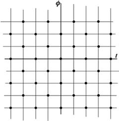
(see Fig. 6.3, middle). From (6.31) and (6.32), we see that the interlaced sampling lattice  is almost twice as sparser as the standard lattice
  . If
. If  , then the interlaced sampling lattice can be obtained from the standard sampling lattice simply by dropping those grid points for which
  is odd (Fig. 6.4). In other words, the same resolution as that of the data measured on the lattice
  can be obtained with only one-half of the data by using the parallel-interlaced scanning geometry. In order to reconstruct data collected over the interlaced lattice, one could first interpolate the missing data to a denser standard lattice and then use (6.23) discretized on this denser lattice. The second approach would be to reconstruct directly from interlaced data (see [9] for error estimates of the corresponding reconstruction).
 (
( ) and the interlaced lattice
  (
( ). In the case of the standard sampling, the replicas of the
  -region are mutually disjoint if
(6.31)

(6.32)
 is almost twice as sparser as the standard lattice
  . If
. If  , then the interlaced sampling lattice can be obtained from the standard sampling lattice simply by dropping those grid points for which
  is odd (Fig. 6.4). In other words, the same resolution as that of the data measured on the lattice
  can be obtained with only one-half of the data by using the parallel-interlaced scanning geometry. In order to reconstruct data collected over the interlaced lattice, one could first interpolate the missing data to a denser standard lattice and then use (6.23) discretized on this denser lattice. The second approach would be to reconstruct directly from interlaced data (see [9] for error estimates of the corresponding reconstruction).
Fig. 6.4
The interlaced lattice (black circles) as a subset of the standard lattice (all intersection points). Both lattices have the same theoretical resolution
Practical application of the parallel-beam geometry can be found, e.g., in SPECT (single-photon emission computer tomography). The parallel-beam geometry of data collected with the SPECT device is a result of the collimation that is required for the correct association of the measured data with lines of integration. It has to be noted that because of the poorness of SPECT data and due to attenuation of the emitted photons in the object on their way to the detector, the FBP algorithm happens to be inappropriate. Different algorithms, mainly from the class of iterative methods, have been developed for the reconstruction of SPECT data (see review [10]).
In transmission tomography, the parallel-beam data can be collected with a pencil beam scanner of the first generation. The corresponding scanning process is a combination of N linear translations of a source-detector system across the object, each made along the line of the predefined orientation. The main disadvantage of this process is that data have to be literally built together in a “sample by sample” fashion, which results in a very long acquisition time.
6.3.2 Fan-Beam Geometry
Collecting fan-beam projections (see Fig. 3.2, left) is preferable in computed tomography because of a much shorter acquisition time compared to that required for the collection of parallel-beam projections.
Thorough derivation of corresponding inversion formulae can be found in [11] and [12]. Below, with minor modifications, we reproduce the derivation shown in [6].
The setup corresponding to a fan-beam geometry is as follows: the source moves around the object in the plane  on the boundary of the disk
  . The center of the disk coincides with the origin of the coordinate system. If
  is the parameter describing the position of the source, then at
  the source is located on the
  -axis. The coordinate system
  defined by (6.7) rotates together with the source.
 on the boundary of the disk
  . The center of the disk coincides with the origin of the coordinate system. If
  is the parameter describing the position of the source, then at
  the source is located on the
  -axis. The coordinate system
  defined by (6.7) rotates together with the source.
As it was mentioned above, Radon data collected with the point source can be efficiently described with parameters either  or
or  (see (6.8) and (6.9) and Fig. 6.2, right). The fan beam, the rays of which are parameterized with ψ, is called equiangular. If the rays within the fan beam are parameterized with Y, the fan beam is said to be equidistant. In both cases, in order to obtain the inversion formulae, the formula (6.23) has to be re-parameterized properly.
 or
or  (see (6.8) and (6.9) and Fig. 6.2, right). The fan beam, the rays of which are parameterized with ψ, is called equiangular. If the rays within the fan beam are parameterized with Y, the fan beam is said to be equidistant. In both cases, in order to obtain the inversion formulae, the formula (6.23) has to be re-parameterized properly.
In order to derive the formula for the inversion of the equidistant fan-beam data, the variables  in the double integral of (6.23) have to be changed for the variables
  according to the transformation:


 in the double integral of (6.23) have to be changed for the variables
  according to the transformation:
(6.33)

(6.34)
Taking into account that

