registration using free-form deformations

which maps any point in the target image I _Ainto its corresponding point in the source image I _B. The transformation $\mathbf{T}$ can be separated into two components: A global component (e.g. a rigid or affine transformation) and a local component. Thus, the transformation $\mathbf{T}$ can be written as:

$\displaystyle{ \mathbf{T}(\mathbf{p}) = \mathbf{T}_{global}(\mathbf{p}) + \mathbf{T}_{local}(\mathbf{p}) }$

(1)

The global transformation typically accounts for variations in the position, orientation and scaling between the two images. However, the global transformation cannot account for any local deformations.

In the late eighties a number of technique for modeling deformations emerged in the computer graphics community. In particular, Sederberg and Parry developed free-form deformations (FFD) [57] as a powerful modelling tool for 3D deformable objects. The basic idea of FFDs is to deform an object by manipulating an underlying mesh of control points. The resulting deformation controls the shape of the 3D object and produces a smooth and continuous transformation. In the original paper by Sederberg and Parry [57] trivariate Bernstein polynomials were used to interpolate the deformation between control points. A more popular choice is to use trivariate B-spline tensor products as the deformation function [37, 38]. The use of FFDs based on B-splines for image registration was first proposed by Rueckert et al. [53, 54]. Over the last decade the use of FFDs for image registration has attracted significant interest [36, 45, 50, 51].

2.1 Free-form deformations

To define a spline-based FFD we denote the domain of the image volume as $\varOmega =\{ \mathbf{p} = (x,y,z)\;\vert \;0 \leq x < X,0 \leq y < Y,0 \leq z < Z\}$ . Let Φ denote a n _x× n _y× n _zmesh of control points ϕ _i, j, kwith uniform control point spacing δ. Then, the FFD can be written as the 3D tensor product of the familiar 1D cubic B-splines:

$\displaystyle{ \mathbf{T}_{local}(\mathbf{p}) =\sum _{ l=0}^{3}\sum _{ m=0}^{3}\sum _{ n=0}^{3}B_{ l}(u)B_{m}(v)B_{n}(w)\phi _{i+l,j+m,k+n} }$

(2)

where $i = \lfloor \frac{x} {\delta } \rfloor - 1,j = \lfloor \frac{y} {\delta } \rfloor - 1,k = \lfloor \frac{z} {\delta } \rfloor - 1,u = \frac{x} {\delta } -\lfloor \frac{x} {\delta } \rfloor,v = \frac{y} {\delta } -\lfloor \frac{y} {\delta } \rfloor,$ $w = \frac{z} {\delta } -\lfloor \frac{z} {\delta } \rfloor$ and where B _lrepresents the l-th basis function of the B-spline [37, 38]:

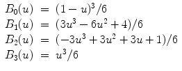$\displaystyle\begin{array}{rcl} B_{0}(u)& =& (1 - u)^{3}/6 {}\\ B_{1}(u)& =& (3u^{3} - 6u^{2} + 4)/6 {}\\ B_{2}(u)& =& (-3u^{3} + 3u^{2} + 3u + 1)/6 {}\\ B_{3}(u)& =& u^{3}/6 {}\\ \end{array}$

In contrast to thin-plate splines [6] or elastic-body splines [23], B-splines are locally controlled which makes them computationally efficient even for a large number of control points. In particular, the basis functions of cubic B-splines have a limited support, i.e. changing control point ϕ _i, j, kaffects the transformation only in the local neighbourhood of that control point.

The derivative of a coordinate transformation is the matrix of its partial derivatives. In the case of 3D coordinate systems this is always a 3 × 3 matrix called the Jacobian matrix and the determinant of this matrix is called the Jacobian determinant of the transformation, or simply the Jacobian. This determinant measures how infinitesimal volumes change under the transformation. For this reason, the Jacobian determinant is the multiplicative factor needed to adjust the differential volume form when applying the coordinate transformation.

An advantage of B-spline FFDs is the fact the derivatives of the transformation can be computed analytically. The derivatives of the transformation are often used in the optimization of the registration and for regularization as well as in the subsequent analysis of the resulting transformation. The Jacobian matrix of transformation is defined as:

$\displaystyle{ \mathbf{J}(\mathbf{p}) = \left (\begin{array}{ccc} \frac{\partial T_{x}(\mathbf{p})} {\partial x} &\frac{\partial T_{x}(\mathbf{p})} {\partial y} &\frac{\partial T_{x}(\mathbf{p})} {\partial z} \\ \frac{\partial T_{y}(\mathbf{p})} {\partial x} &\frac{\partial T_{y}(\mathbf{p})} {\partial y} &\frac{\partial T_{y}(\mathbf{p})} {\partial z} \\ \frac{\partial T_{z}(\mathbf{p})} {\partial x} & \frac{\partial T_{z}(\mathbf{p})} {\partial y} & \frac{\partial T_{z}(\mathbf{p})} {\partial z}\\ \end{array} \right ) }$

(3)

The determinant of this matrix measures how infinitesimal volumes change under the transformation and can be used to analyze the local behavior of the transformation. A positive value of the determinant of the Jacobian matrix can be interpreted as follows:

$\displaystyle{ J(\mathbf{p}) =\det \vert \mathbf{J}(p)\vert = \left \{\begin{array}{ll} > 1&\mbox{ volume expansion} \\ = 1&\mbox{ no volume change} \\ < 1&\mbox{ volume contraction} \end{array} \right. }$

(4)

If the value of the determinant changes from positive to negative the transformation is folding and is no longer a one-to-one transformation. Since the FFD is the tensor product of independent 1D B-splines, the derivative of the local transformation $\mathbf{T}_{local}$ with respect to x is computed as follows:

$\displaystyle{ \frac{\partial \mathbf{T}_{local}(\mathbf{p})} {\partial x} = \frac{1} {\delta _{x}}\sum _{l=0}^{3}\sum _{ m=0}^{3}\sum _{ n=0}^{3}\frac{dB_{l}(u)} {du} B_{m}(v)B_{n}(w)\phi _{i+l,j+m,k+n} }$

(5)

The remaining derivatives have an analogous form. The computation of the derivatives of the B-spline basis functions B _iitself is straightforward.

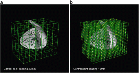
The control points Φ act as parameters of the B-spline FFD and the degree of non-rigid deformation which can be modelled depends essentially on the resolution of the mesh of control points Φ. A large spacing of control points allows modelling of global non-rigid deformations while a small spacing of control points allows modelling of highly local non-rigid deformations. At the same time, the resolution of the control point mesh defines the number of degrees of freedom and consequently the computational complexity. A common approach uses a multi-resolution approach for FFDs in which the resolution of the control point mesh is increased in a coarse to fine fashion (see Fig. 1). An arbitrary FFD based on B-splines can be refined to an identical deformation with half the control point spacing along each dimension. In the 1D case, the control point positions ϕ′ of the refined grid can be computed from the coarse control points ϕ [26]:

$\displaystyle{ \phi _{2i+1}' = \frac{1} {2}(\phi _{i} +\phi _{i+1})\quad \mbox{ and}\quad \phi _{2i}' = \frac{1} {8}(\phi _{i-1} +\phi _{i+1} + 6\phi _{i}) }$

(6)

This equation can be easily generalized to 3D by applying the tensor product. Another possibility is the use of non-uniform FFDs [55]. This can be achieved by introducing a control point status associated with each control point in the mesh, marking it either active or passive. Active control points can be modified during the registration process, whereas passive control points remain fixed. An alternative approach for FFDs based on non-uniform rational B-splines (NURBS) has been proposed by Wang and Jiang [64].

Fig. 1

A free-form deformation control point mesh (a) before subdivision (control point spacing 20 mm) and (b) after subdivision (control point spacing 10 mm)

In general FFDs are defined on a Cartesian coordinate system, however it is possible to use other coordinate systems. For example, Chandrashekara proposed the use of a FFD model defined in a cylindrical coordinate system for the registration of cardiac MR images [11]. In a similar fashion, Lin et al. [40] proposed the use of extended free-form deformations (EFFD) [19] for the registration of cardiac MR images. Another, more generic, approach has been recently proposed by Chandrashekara [10]: In this approach free-form deformations are defined on lattices with arbitrary topology [42]. An advantage of this approach is the fact that the control point mesh can be closely adapted to the geometry of the anatomy studied, e.g. epi- and endocardial surfaces of the left ventricle.

2.2 Voxel-based similarity measures for free-form deformations

To relate a point in the target image to the source image, one must define a similarity criterion (or cost function) which measures the degree of alignment between both images. A popular choice for this are voxel-based similarity measures which use the image intensities directly and do not require the extraction of any features such as a landmarks, curves or surfaces. Commonly used voxel-based similarity measures include the sum of squared differences (SSD) or cross-correlation (CC). However, these measures make rather strong assumptions about the relationship of the image intensities in both images which is not suitable for multi-modality registration. Even in the case of mono-modality registration this assumption is often violated, e.g. in contrast-enhanced imaging. An alternative voxel-based similarity measure is mutual information (MI) which was independently proposed by Collignon [16] and Viola [62]. Mutual information is based on the concept of information theory and expresses the amount of information in one image A that explains a second image B,

$\displaystyle{ \mathcal{C}_{\mathit{similarity}}(A,B) = H(A) + H(B) - H(A,B) }$

(7)

where H(A), H(B) denote the marginal entropies of A, B and H(A, B) denotes their joint entropy. These entropies can be estimated from the joint histogram of A and B or using kernel density estimators like Parzen windowing. If both images are aligned the mutual information is maximised. It has been shown by Studholme [60] that mutual information itself is not independent of the overlap between two images. To avoid any dependency on the amount of image overlap, Studholme suggested the use of normalised mutual information (NMI) as a measure of image alignment:

$\displaystyle{ \mathcal{C}_{\mathit{similarity}}(A,B) = \frac{H(A) + H(B)} {H(A,B)} }$

(8)

Similar forms of normalised mutual information have been proposed by Maes et al. [43]. A more complete review of the use of mutual information for image registration can be found in [48].

2.3 Optimization of free-form deformations

Like many other problems in computer vision, registration can be formulated as an optimisation problem whose goal is to minimise an associated energy or cost function. The most general form of such a cost function in registration is

$\displaystyle{ \mathcal{C} = -\mathcal{C}_{\mathit{similarity}} +\lambda \mathcal{C}_{\mathit{penalty}} }$

(9)

This type of cost function comprises two competing goals: The first term represents the cost associated with the image similarity $\mathcal{C}_{\mathit{similarity}}$ in Eqs. (7) or (8) while the second term penalizes certain transformations and thus constrains the behavior of the transformation (different penalty functions will be discussed in the next section). The parameter λ is a weighting parameter which defines the trade-off between the alignment of the two images and the penalty function of the transformation. From a probabilistic point of view, the cost function in Eq. (9) can be explained in a Bayesian context: The similarity measure can be viewed as a likelihood term which expresses the probability of a match between source and target image while the penalty function represents a prior which encodes a-priori knowledge about the expected transformation.

In the original paper by Rueckert et al. [54] the optimization of the FFD is carried out is a multi-resolution fashion via a steepest gradient descent optimization algorithm. More recently, Klein et al. has compared different optimization strategies for FFDs [35].

2.4 Penalty functions for free-form deformations

Typically, non-rigid image registration is an ill-posed problem. Thus, it is necessary to add some constraints to render the problem well-posed. A common approach is enforce the smoothness of the deformation [54]. Free-form deformations based on B-splines are intrinsically smooth (at least relative to the control point spacing), however additional smoothness can be enforced by adding a penalty term which regularizes the transformation. The general form of such a smoothness penalty term has been described by Wahba [63]. In 3D, the penalty term takes the following form

$\displaystyle\begin{array}{rcl} \mathcal{C}_{\mathit{smooth}}& =& \int \limits \left (\frac{\partial ^{2}\mathbf{T}} {\partial x^{2}} \right )^{2}\!\! + \left (\frac{\partial ^{2}\mathbf{T}} {\partial y^{2}} \right )^{2}\!\! + \left (\frac{\partial ^{2}\mathbf{T}} {\partial z^{2}} \right )^{2}\!\! \\ & & +\ 2\left (\frac{\partial ^{2}\mathbf{T}} {\partial xy}\right )^{2}\!\! + 2\left (\frac{\partial ^{2}\mathbf{T}} {\partial xz} \right )^{2}\!\! + 2\left (\frac{\partial ^{2}\mathbf{T}} {\partial yz} \right )^{2}d\mathbf{p}{}\end{array}$

(10)

This quantity is the 3D counterpart of the 2D bending energy of a thin-plate of metal and defines a cost function which is associated with the smoothness of the transformation. Note that this regularization term is zero for an affine transformation and therefore penalises only non-affine transformations [63].

Another class of penalty functions aim to generate biomechanically plausible deformations. For example, Rohlfing et al. suggested a constraint which preserves volume [51]:

$\displaystyle{ \mathcal{C}_{\mathit{volume}} =\int \limits \left \vert \log (J(\mathbf{p}))\right \vert d\mathbf{p} }$

(11)

Here $J(\mathbf{p})$ is the determinant of the Jacobian matrix $\mathbf{J}$ of the free-form deformation. As mention previously the Jacobian measures how infinitesimal volumes change under the transformation. This function therefore penalizes the compression or expansion of tissues or organs during the registration. It should be noted that the penalty term above penalizes volume changes over the entire domain, however due to the integration there may be small regions in the image which show a large volume change while the majority of regions show no volume change. Other authors have proposed a rigidity constraint which forces the deformation in certain regions to be nearly rigid [41], e.g.

$\displaystyle{ \mathcal{C}_{\mathit{rigidity}} =\int \limits \vert \vert \mathbf{J}(\mathbf{p})\mathbf{J}(\mathbf{p})^{T} -\mathbf{1}\vert \vert d\mathbf{p} }$

(12)

The penalty functions above do not guarantee that the resulting deformation field is diffeomorphic (smooth and invertible). In order to ensure that the FFD is diffeomorphic it is possible to add a penalty function which penalizes non-diffeomorphic transformations, e.g. transformations which introduce folding. One suitable penalty function for this has the following form:

$\displaystyle{ \mathcal{C}_{\mathit{folding}} =\int \limits \mathcal{P}(\mathbf{p})d\mathbf{p}\ }$

(13)

where

$\displaystyle{ \mathcal{P}(\mathbf{p}) = \left \{\begin{array}{ll} \frac{\gamma ^{2}} {\vert (J(\mathbf{p})\vert ^{2}} - 2&\mbox{ if }\vert J(\mathbf{p})\vert \leq \gamma \\ 0 &\mbox{ otherwise} \end{array} \right. }$

(14)

A similar penalty function was first proposed by Edwards et al. [25] and effectively penalises any transformations for which the determinant of the Jacobian falls below a threshold γ. By penalising Jacobians that approach zero, one can prevent the transformation from collapsing and ensure diffeomorphisms. Note that simply using a smoothness penalty function would not be sufficient to guarantee a diffeomorphic transformation, since it is possible for a transformation to be smooth but non-diffeomorphic.

2.5 Diffeomorphic free-form deformations

In general, most registration algorithms make the assumption that similar structures are present in both images. Therefore it is desirable that the deformation field be smooth and invertible (so that every point in one image has a corresponding point in the other). Such smooth, invertible transformations are called diffeomorphisms. Choi and Lee [13] have derived sufficient conditions for the injectivity of FFDs which are represented in terms of control point displacements. These sufficient conditions can be easily tested and can be used to guarantee a diffeomorphic FFD. Without loss of generality we will assume in the following that the control points are arranged on a lattice with unit spacing. Let $\varDelta \mathbf{c}_{i,j,k} = (\varDelta x_{i,j,k},\varDelta y_{i,j,k},\varDelta z_{i,j,k})$ be the displacement of control point c _i, j, k. Let $\delta _{x} =\max \vert \varDelta x_{i,j,k}\vert$ , $\delta _{y} =\max \vert \varDelta y_{i,j,k}\vert$ , $\delta _{z} =\max \vert \varDelta z_{i,j,k}\vert$ .

Theorem 1.

A FFD based on cubic B-splines is locally injective over all the domain if $\delta _{x} < \frac{1} {K}$ , $\delta _{y} < \frac{1} {K}$ and $\delta _{z} < \frac{1} {K}$ .

Only gold members can continue reading. Log In or Register to continue