and  be two images that are geometrically related by the registration transformation
  with parameters
  such that voxels p in
  with intensity a correspond to voxels
  in
in  with intensity b. Taking random samples p in
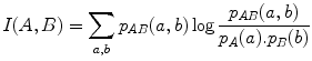
  , a and b can be considered as discrete random variables A and B with joint and marginal distributions p A B (a, b), p A (a) and p B (b) respectively. The mutual information I(A, B) of A and B measures the degree of dependence between A and B as the distance between the joint distribution p A B (a, b) and the distribution associated to the case of complete independence p A (a). p B (b), by means of the Kullback-Leibler measure [4], i.e.
(1)
 , i.e. on the registration of the images. The mutual information registration criterion postulates that the images are geometrically aligned by the transformation
  for which I(A, B) is maximal:
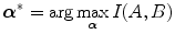
Mutual information is related to the information theoretic notion of entropy by the equations  with H(A) and H(B) being the entropy of A and B respectively, H(A, B) their joint entropy and H(A | B) and H(B | A) the conditional entropy of A given B and of B given A respectively. The entropy H(A) is a measure of the amount of uncertainty about the random variable A, while H(A | B) is the amount of uncertainty left in A when knowing B. Hence, I(A, B) measures the amount of information that one image contains about the other, which should be maximal at registration. If both marginal distributions p A (a) and p B (b) can be considered to be independent of the registration parameters
  , the MI criterion reduces to minimizing the joint entropy H A B (A, B). If either p A (a) or p B (b) is independent of
  , which is the case if one of the images is always completely contained in the other, the MI criterion reduces to minimizing the conditional entropy H(A | B) or H(B | A). However, if both images only partially overlap, which is very likely during optimization, the volume of overlap will change when
  is varied and both marginal distributions p A (a) and p B (b) and therefore also their entropies H(A) and H(B) will in general depend on
  . Hence, maximizing mutual information will tend to find as much as possible of the complexity that is in the separate data sets so that at the same time they explain each other well.
with H(A) and H(B) being the entropy of A and B respectively, H(A, B) their joint entropy and H(A | B) and H(B | A) the conditional entropy of A given B and of B given A respectively. The entropy H(A) is a measure of the amount of uncertainty about the random variable A, while H(A | B) is the amount of uncertainty left in A when knowing B. Hence, I(A, B) measures the amount of information that one image contains about the other, which should be maximal at registration. If both marginal distributions p A (a) and p B (b) can be considered to be independent of the registration parameters , the MI criterion reduces to minimizing the joint entropy H A B (A, B). If either p A (a) or p B (b) is independent of , which is the case if one of the images is always completely contained in the other, the MI criterion reduces to minimizing the conditional entropy H(A | B) or H(B | A). However, if both images only partially overlap, which is very likely during optimization, the volume of overlap will change when is varied and both marginal distributions p A (a) and p B (b) and therefore also their entropies H(A) and H(B) will in general depend on . Hence, maximizing mutual information will tend to find as much as possible of the complexity that is in the separate data sets so that at the same time they explain each other well.Other information-theoretic registration measures can be derived from the MI criterion presented above, such as the entropy correlation coefficient 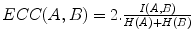 [19] or the normalized mutual information
 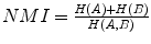 [38] with 0 ≤ E C C ≤ 1, 1 ≤ N M I ≤ 2 and
 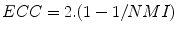 . Maximization of N M I or E C C may be superior to MMI itself in case the region of overlap of both images is relatively small at the correct registration solution, as MMI may be biased towards registration solutions with larger total amount of information H(A) + H(B) within the region of overlap [38]. MI is only one example of the more general f − i n f o r m a t i o n measures of dependence, several of which were investigated for image registration in [31].
[19] or the normalized mutual information [38] with 0 ≤ E C C ≤ 1, 1 ≤ N M I ≤ 2 and . Maximization of N M I or E C C may be superior to MMI itself in case the region of overlap of both images is relatively small at the correct registration solution, as MMI may be biased towards registration solutions with larger total amount of information H(A) + H(B) within the region of overlap [38]. MI is only one example of the more general f − i n f o r m a t i o n measures of dependence, several of which were investigated for image registration in [31].4 Implementation
The MMI registration criterion does not require any preprocessing or segmentation of the images. With each of the images is associated a 3-D coordinate frame in millimeter units, that takes the pixel size, inter-slice distance and the orientation of the image axes relative to the patient into account. One of the images to be registered is selected to be the floating image  from which samples s ∈ S are taken and transformed by the geometric transformation
  with parameters
  into the reference image
  . S may include all voxels in
  or a subset thereof to increase speed performance.
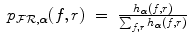
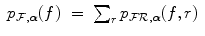
from which samples s ∈ S are taken and transformed by the geometric transformation with parameters into the reference image . S may include all voxels in or a subset thereof to increase speed performance.The MMI method requires the estimation of the joint probability density p(f, r) of corresponding voxel intensities f and r in the floating and reference image respectively. This can be obtained from the joint intensity histogram of the region of overlap of the images. The joint image intensity histogram  of the volume of overlap
  of
of  and
and  can be constructed by simple binning of the image intensity pairs
 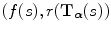 for all
  . In order to do this efficiently, the floating and the reference image intensities are first linearly rescaled to the range
 ![$$[0,n_{\mathcal{F}}- 1]$$](/wp-content/uploads/2016/09/A151032_1_En_16_Chapter_IEq30.gif) and
and ![$$[0,n_{\mathcal{R}}- 1]$$](/wp-content/uploads/2016/09/A151032_1_En_16_Chapter_IEq31.gif) respectively, with
respectively, with  and
and  the number of bins assigned to the floating and reference image respectively and
  being the total number of bins in the joint histogram. Estimations for the marginal and joint image intensity distributions
  ,
,  and
and  are obtained by normalization of
and the MI registration criterion is evaluated using
of the volume of overlap of and can be constructed by simple binning of the image intensity pairs for all . In order to do this efficiently, the floating and the reference image intensities are first linearly rescaled to the range and respectively, with and the number of bins assigned to the floating and reference image respectively and being the total number of bins in the joint histogram. Estimations for the marginal and joint image intensity distributions , and are obtained by normalization of (2)
(3)
(4)
(5)
Typically,  and
and  need to be chosen much smaller than the number of different values in the original images in order to assure a sufficient number of counts in each bin. If not, the joint histogram
  would be rather sparse with many zero entries and entries that contain only one or a few counts, such that a small change in the registration parameters
  would lead to many discontinuous changes in the joint histogram, with non-zero entries becoming zero and vice versa, that propagate into
  . Such abrupt changes in
  induce discontinuities and many local maxima in
  , which deteriorates optimization robustness of the MI measure. Appropriate values for
  and
and  can only be determined by experimentation. Moreover,
  will in general not coincide with a grid point of
  , such that interpolation of the reference image is needed to obtain the image intensity value
  . Zeroth order or nearest neighbor interpolation of
  is most efficient, but is insensitive to translations up to 1 voxel and therefore insufficient to guarantee subvoxel accuracy. But even when higher order interpolation methods are used, such as linear, cubic or B-spline interpolation, simple binning of the interpolated intensity pairs (f(s), r(T α s)) leads to discontinuous changes in the joint intensity probability
  and in the marginal probability
  for small variations of α when the interpolated values r(T α s) fall in a different bin. Note that post-processing the histogram obtained by binning by convolution with a Gaussian or other smoothing kernel is not sufficient to eliminate these discontinuities.
and need to be chosen much smaller than the number of different values in the original images in order to assure a sufficient number of counts in each bin. If not, the joint histogram would be rather sparse with many zero entries and entries that contain only one or a few counts, such that a small change in the registration parameters would lead to many discontinuous changes in the joint histogram, with non-zero entries becoming zero and vice versa, that propagate into . Such abrupt changes in induce discontinuities and many local maxima in , which deteriorates optimization robustness of the MI measure. Appropriate values for and can only be determined by experimentation. Moreover, will in general not coincide with a grid point of , such that interpolation of the reference image is needed to obtain the image intensity value . Zeroth order or nearest neighbor interpolation of is most efficient, but is insensitive to translations up to 1 voxel and therefore insufficient to guarantee subvoxel accuracy. But even when higher order interpolation methods are used, such as linear, cubic or B-spline interpolation, simple binning of the interpolated intensity pairs (f(s), r(T α s)) leads to discontinuous changes in the joint intensity probability and in the marginal probability for small variations of α when the interpolated values r(T α s) fall in a different bin. Note that post-processing the histogram obtained by binning by convolution with a Gaussian or other smoothing kernel is not sufficient to eliminate these discontinuities.Related posts:

Stay updated, free articles. Join our Telegram channel

Full access? Get Clinical Tree


