15 The main goal of this chapter is to explain design and analysis issues that can influence sample size estimation, including: • Descriptive studies (one-sample) • Comparative studies (two or more samples) • Continuous/measured outcomes • Dichotomous outcomes • Diagnostic tests • Reliability studies An important aspect of study design and analysis is sample size. An appropriate sample size achieves certain desirable properties for statistical inferences including descriptive (one-sample) and comparative (two-sample) studies. These can either be for the purpose of estimation of unknown parameters or testing. Table 15.1 briefly reports descriptive and comparative quantities of interest which are suitable for sample size calculations. Sample size is influenced by three major factors: (1) design features, (2) analysis features, and (3) logistics as they shape the problem at hand. Analysis is the focus in this chapter, as design has been previously discussed and logistics are realities that should be incorporated into design and, to an extent, analysis. Table 15.2 provides a brief summary of the three factors. Table 15.1 Categorization of various quantities of interest, suitable for sample size calculations
Sample Size Estimation
 Learning Objectives
 Concepts
| Descriptive | Comparative |
Binary | Proportion | RD, OR, RR, HR, etc. |
Continuous | Mean | Mean difference, correlation coefficient, etc. |
Abbreviations: RD, risk difference; OR, odds ratio; RR, relative risk; HR, hazard ratio.
The motivation for sample size calculations is often to achieve one of two major goals: avoid exceeding a maximum acceptable (as scientifically meaningful) width for a confidence interval, or achieve a predefined power for a study. Intuitively, one should expect that larger sample sizes provide more information and, thus, yield better estimates (narrower confidence intervals) leading to correct decisions in hypothesis tests (adequate power). One enhances the accuracy of estimation through confidence intervals, and the other increases the study power. In either case, the study could be descriptive (one sample) or comparative (two or more groups). Each of these features in various combinations is discussed with examples throughout the chapter.
Sample Size Estimation Based on Confidence Intervals
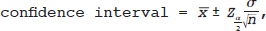
The first sample size calculations described are those relating to confidence intervals. The general form of a confidence interval for the true mean is given by the following formula:
where  is the sample mean,
  is the (positive) critical value from the normal distribution corresponding to the 100 (1 − α)% confidence interval, σ is the population standard deviation, and n is the size of the sample. From this formula one can tell that the interval is centered around
  , and extends a length
  in both directions from the center, giving a width of
  . The width decreases with increasing values of n. Instead of discussing the full width of the interval, it is common to discuss just the half-width of intervals,
  , how far the interval extends from the center, and is called the margin of error. Therefore, the confidence interval can then be written as
Table 15.2 Factors influencing sample size
Design | Analysis | Logistics |
• Cross-sectional/cohort/case-control | • Scale of outcome | • Drop-out |
• Descriptive/analytical | • Effect measure | • Missing data |
• Parallel/cross-over | • Confidence interval | • Funding |
• Repeated measures | • Test of hypothesis | • Nature of disease |
• Bioequivalence | • Directional vs. nondirectional | • Scope of survey |
• Adjustment for confounders |
|
|

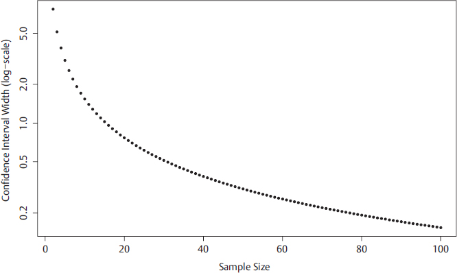
Both the margin of error and the width of the interval decrease proportionally with  , as illustrated in Fig. 15.1.
Note that this interval width decreases toward 0 as the size of the study sample increases. If m represents the margin of error of the confidence interval, one can very simply rearrange the formula to obtain
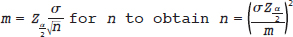
Here, the impact of various factors on sample size is explicit. In particular, to achieving a small margin of error, m, requires a large sample size, n. There are two other major components which impact the width of a confidence interval: the total remaining tail area outside of the interval which defines the confidence interval, α, and the standard error  (when the central limit theorem is used). The standard error itself is obviously impacted by the standard deviation of the population, σ, and the sample size, n.
Sample Size Estimation Based on Hypothesis Tests (One-sided)
Hypothesis testing can be another focus for estimating an appropriate sample size for a study. Recall that power is the probability of rejecting the null hypothesis when it is indeed false, and so it is desirable for this to be as close to 100% as much as possible. If investigators use the normal distribution and a predefined power that they were interested in achieving for their study, then the formula for sample size is
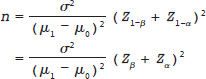
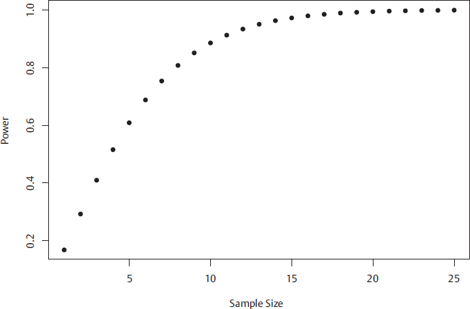
where Z1−β is the critical value associated with the power 1 − β (β is the probability of making a type 2 error), and μ1 is the “true” mean used to estimate the detectable effect size of interest from the hypothesized mean, μ1 − μ0, and other symbols denote the same quantities as in confidence intervals. Here, one sees that the sample size is influenced as before by the variance of the population, σ2, namely larger variances demand larger sample sizes, but also by the effect size of interest to detect, and the power. The larger the effect size of interest, the easier it should be to detect, so larger effect sizes decrease the required sample size. Finally, larger values of power correspond to larger values (in magnitude) of Zβ so this extra certainty in testing requires greater sample size. Fig. 15.2 illustrates the sample size required for a one-tailed test where the null hypothesis is that the true mean, μ, is equal to the hypothesized mean, μ0: μ = μ0 when in truth μ = μ1 ≠ μ0 for some μ1.
Unlike the one-sided hypothesis test, there is no formula in the form n = … for sample size for two-sided tests. Instead, numerical approximations calculated by software are used. These will be investigated directly within examples and exercises.
Variants of formulae for estimating appropriate sample size scenarios are discussed in this chapter, including when standard deviation is estimated rather than known for continuous measurements (using the t distribution rather than a normal), when the outcome is binary, and performing inference on proportions (using the normal distribution suitable approximations when proportions of interest are not near 0 or 1). Other variants of formulae for sample size estimation arise by making adjustments in the estimate for standard error. The number of variants beyond a simple case is too large to cover exhaustively in this chapter, and usually involve calculations that are tedious, although not difficult. For these and other scenarios, existing software is particularity useful. In this chapter some of the formulae and theory behind these concepts are omitted in favor of illustrating solutions provided by R functions.
Diagnostic Test Performance Sample Size Calculations
For sample size estimations of the area-under-the-curve (AUC) and reliability of diagnostic test readings, one should refer to the results of existing methodological work. Because of the more involved calculations, approximations are often used for such estimations. This chapter illustrates approaches that are implemented in R as well as approaches that use tables. Some of these tables, and the means of constructing tables, have been described elsewhere.1
Reliability can be measured by different ways, and so the sample size calculations for each can differ. For example, hypothesis testing on AUCs can be used to assess whether two raters are indicating that the same images are abnormal. The appropriate hypothesis test for this scenario is the Wilcoxon rank sum test,2,3 measuring if one rater ranks images “higher” than another rater, beyond what is expected due to chance. In an example in musculoskeletal imaging, the raters may assess the same images and assign a score to each case according to the amount of cartilage degeneration in the joint. If classifying a set of images to only two categories (e.g., “normal” or “abnormal”), two raters may agree by chance and this should be incorporated into calculations. The interrater agreement between two raters when rating images dichotomously can be measured by Cohen’s kappa coefficient,4 which achieves a value of 1 if the two raters completely agree and a value of 0 if the raters only agree as much as expected simply due to chance. If there are more than two possible classifications, say raters are rating the severity on something more like a Likert scale, the intraclass correlation coefficient (ICC) is suitable. The ICC is a ratio (proportion) of variances: the variance between images compared to the total variance, and is the same idea as an ANOVA. If this ratio is close to 1, then most of the variation in ratings is because of the variety of images, meaning that very little is due to variation between raters. The ICC, being a proportion, lies between 0 and 1, but has more sophisticated calculations for sample size as this measures more than just a simple frequency. When incorporating power the numerical methods are also difficult. Although exact methods have been found5 a useful approximation may be more feasible in practice and only requires reading off published tables.1 For reliability measured with kappa or ICC, software and tables are referred over formulae.
 Examples Estimating Sample Size
This section exclusively covers a variety of sample size calculations in a variety of contexts. As noted, this is not an exhaustive list but covers many of the concepts used in sample size calculations.
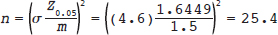
Example 1: Target Confidence Interval Width for Count Outcome
Consider a study in which investigators aim to determine the number of metastatic lesions that are detected in the liver in patients with advanced pancreatic cancer by contrast-enhanced CT. The standard deviation of number of lesions per patient is 4.6. On the basis of this standard deviation, what sample size is required for the investigators to construct a 90% confidence interval for the true mean with a margin of error no more than 1.5 lesions per patient?
Solution: The solution in this case only requires substituting parameters by numbers into the formula: