Data Acquisition of Emission Tomographyn
Conventional or planar radionuclide imaging suffers a major limitation in the loss of object contrast as a result of background radioactivity. In the planar image, radioactivity underlying and overlying the object of interest is superimposed on that coming from the object. The fundamental goal of tomographic imaging systems is a more accurate portrayal of the three-dimensional (3D) distribution of radioactivity in the patient, with improved image contrast and definition of image detail. This is analogous to the way computed tomography (CT) provides better soft tissue contrast than planar radiography. The Greek tomo means “to cut”; tomography may be thought of as a means of “cutting” the body into discrete image planes. Tomographic techniques have been developed for both single-photon and positron imaging, referred to as single-photon emission computed tomography (SPECT) and positron emission tomography (PET), respectively.
Restricted or limited-angle tomography keeps the plane of interest in focus while blurring the out-of-plane data in much the same way as conventional x-ray tomography. Various restricted-angle systems have been investigated, including multi-pinhole collimator systems, pseudo-random, coded-aperture collimator systems, and various rotating slant-hole collimator systems. Although clinical use has been limited, resurgent interest has been shown for specific imaging applications, including those designed for cardiac and breast imaging.
Tomographic approaches that acquire data over 180 or 360 degrees provide a more complete reconstruction of the object and therefore are more widely used. Rotating gamma camera SPECT systems offer the ability to perform true transaxial tomography. PET uses a method called annihilation coincidence detection to acquire data over 360 degrees without the use of absorptive collimation. The most important characteristic of these approaches is that only data arising in the image plane of interest are used in the reconstruction of the tomographic image. This is an important characteristic leading to improved image contrast compared with methods using restricted-angle tomography. As will be discussed, the reconstruction of these data has historically been done with filtered back-projection. However, iterative techniques such as ordered subsets expectation maximization (OSEM) are increasingly used. This chapter reviews the current approaches to the acquisition and reconstruction of SPECT and PET, including the use of hybrid imaging such as PET/CT, PET/MR and SPECT/CT, and the quality control necessary to ensure high-quality clinical results.
All tomographic modalities used in diagnostic imaging, including SPECT, PET, CT, and magnetic resonance imaging (MRI), acquire raw data in the form of projection data at a variety of angles about the patient. Although SPECT and PET use different approaches to acquiring these data, the nature of the data is essentially the same. Image reconstruction involves the processing of these data to generate a series of cross-sectional images through the object of interest.
The geometries associated with the acquisition of SPECT and PET are illustrated in Fig. 3.1 . In the simple SPECT example using a parallel-hole collimator, the data acquired at a particular location in the gamma camera crystal originated from a line passing through that point perpendicular to the surface of the sodium iodide (NaI) crystal face and is referred to in the figure as the line of origin (see Fig. 3.1 , left ). Thus the data at this point can be seen to represent the sum of counts that originated along this line, or ray, referred to as a ray sum. These ray-sum values across the patient are referred to as the projection data for this cross-sectional slice at this particular viewing angle. For PET, the ray sum represents the data collected along a particular line of response (LOR) connecting a pair of detectors involved in a coincidence detection event (see Fig. 3.1 , right ).

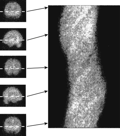
For a SPECT acquisition, the projection image acquired at each angle consists of the stack of projections for all slices within the camera field of view at that angle. Fig. 3.2 , on the right, shows projections from a SPECT brain scan at five different viewing angles. For a particular slice (see Fig. 3.2 , dashed white line ), a row of the projection data for each angle can be stacked such that the displacement along the projection is on the x -axis and the viewing angle is on the y -axis (see Fig. 3.2 , right ). This plot is referred to as the sinogram , because the resulting plot of a point source resembles a sine-wave plot turned on its side. A more complicated object such as a brain scan can be perceived as many such sine waves overlaid on top of each other for each point within the object. The sinogram, represents the full set of projection data necessary to reconstruct a particular single slice. A separate slice is made in the sinogram for each cross-sectional slice through the object. The set of projection views and the set of sinograms are alternative means of displaying the projection data associated with a tomographic acquisition. Each projection view displays the projection data across all slices with a separate image for each angle, whereas the sinogram displays the projection data across all angles with a separate sinogram for each slice.
The geometry of PET acquisition (see Fig. 3.1 , right ) involves the data acquired along a particular LOR connecting two detectors that may be involved in an annihilation coincidence detection event. These data thus represent the ray sum along this LOR. The data associated with a particular LOR are characterized in the sinogram by their distance from the center of the gantry (on the x -axis) and their angle of orientation (on the y -axis). In this manner, PET data acquisition directly into sinograms may be more straightforward than into projection views. In a PET detection event, the two detectors involved in the coincidence event are identified, and the LOR is recorded. The location in the sinogram corresponding to that particular LOR is localized, and its data are incremented. After the collection of many such events, the projection data are represented by a set of sinograms for each PET slice. However, these data also can be displayed as projection views similar to those acquired in SPECT studies. This simple example illustrates the acquisition of PET data in 2D mode, in which each cross-sectional slice basically is acquired separately. Most current PET scanners acquire data only in 3D mode, in which LORs cut across the parallel cross-section slices. The corresponding projection data will include oblique views or sinograms through the object. With time-of-flight PET (discussed later in this chapter), it is necessary to record not only the LOR but also the time difference between the two detections involved in the annihilation coincidence detection event, which will also be incorporated into the reconstruction of these data.
Tomographic data can be acquired in a dynamic or gated approach. For example, a PET study can be acquired as a time sequence of scans that might be simple or multiphase (e.g., ten 5-second frames, four 30-second frames, and five 60-second frames). In addition, the tomographic study can be acquired in association with a physiological gate such as the electrocardiogram (ECG) or a respiratory signal. For example, myocardial perfusion SPECT is acquired in conjunction with the ECG. In dynamic or gated tomographic acquisitions, a full set of projection data acquired at each time or gate point is to be reconstructed separately.
Tomographic Reconstruction
Images, like time signals, can be considered as either a spatial variation of the signal or a sum of signals of varying frequencies. It is intuitive to consider images as a spatial variation in the signal because some part of the image will be bright and other parts will be dark. In nuclear medicine, the bright and dark areas may correspond to regions of high and low radiopharmaceutical uptake, respectively. Conversely, it is not intuitive to consider an image to comprise signals of varying frequency, although this is in fact the case. On the other hand, we do naturally perceive audio signals in terms of frequencies. A choral performance comprises sopranos, altos, tenors, and basses, and the combination of these voices hopefully leads to a very pleasurable experience. On the other hand, we cannot perceive a presentation of the audio signal as a temporal variation of the signal and intuitively identify it as music. The music is fully described by either representation, and there may be cases in which either the temporal (i.e., real) or the frequency representation is the best approach for considering the audio data. The same is true for image data, except the variations are in space rather than time.
Image data may be best represented in either spatial (real) or frequency space. The mathematician Joseph Fourier noted in 1807 that any arbitrary signal can be generated by adding a large number of sine and cosine signals of varying frequencies and amplitudes. The plot of amplitude as a function of frequency is referred to as the Fourier transform, and it defines the components of the image at each frequency. The low frequencies provide the overall shape of the object, whereas the high frequencies help define the sharp edges and fine detail within the image. Audio signals can be manipulated by emphasizing certain frequencies (low or high); the same is true for images. Image noise is typically present in all frequencies; if the low frequencies are emphasized, the image may be less noisy but blurry, whereas emphasizing the high frequencies will accentuate both the edges of the objects and the noise. Such image manipulation is referred to as filtering because it allows certain spatial frequencies to be realized while removing others.
Since the initial development of CT 40 years ago, filtered back-projection has been the most common approach to reconstructing medical tomographic data, including SPECT, PET, and CT, although iterative techniques were introduced into the clinic for use with PET more than a decade ago. However, filtered back-projection is still used in SPECT and remains the most common method for CT. In back-projection, it is assumed that all of the data detected at a particular point along the projection originated from somewhere along the line emanating from this point. For SPECT using parallel-hole collimation, this would be the line of origin passing through the detection point and perpendicular to the NaI crystal surface. For PET, events would be assumed to have come from the LOR connecting the two detectors involved in the annihilation coincidence detection event. In general, back-projection makes no assumptions of where along the line the event occurred, and thus the counts are spread evenly along the line. In other words, the counts are back-projected along the line of origin or LOR. All of the counts from every location along every projection are back-projected across the reconstructed image ( Fig. 3.3, A ). The result is referred to as simple back-projection; it has substantial streak artifacts that, in all but the simplest objects, render the reconstructed image indiscernible (see Fig. 3.3, B ). These streaks are caused by uneven sampling of frequency space during the back-projection process, where low frequencies are sampled at a much higher rate than higher frequencies. To compensate for this, a filter, called the ramp filter, is applied during the reconstruction that increases linearly with frequency ( Fig. 3.4 ). Applying back-projection in conjunction with such filtration is referred to as filtered back-projection. With a very large number of accurate, noiseless projections, filtered back-projection will yield an excellent, almost perfect reconstruction.

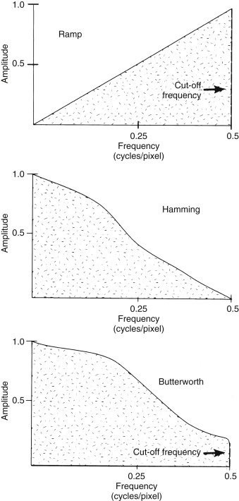
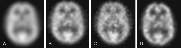
However, with true clinical data, the projections are noisy, and thus the ramp filter will tend to accentuate the high-frequency noise in the data. Therefore a windowing filter is applied, in addition to the ramp filter, to smoothly bring the filter back to zero at frequencies above the pertinent content in the study. Commonly used windowing functions include the Hamming and Butterworth filters (see Fig. 3.4 ). With these filters, a cutoff frequency is defined, which is the point at which they return to zero, with no higher frequencies being incorporated into the reconstructed image. Noting that low frequencies yield the overall shape and high frequencies yield the sharp edges and fine detail, the appearance of the resultant reconstructed image can be altered by varying the cutoff frequency. Selecting a cutoff frequency that is too low will yield a blurry reconstruction ( Fig. 3.5, A , far left ), and one that is too high will yield a noisy reconstruction (see Fig. 3.5, C , second from the right ). However, an appropriate choice for cutoff frequency will provide an image that is a fair compromise between noise and detail (see Fig. 3.5, B, second from left ). With an appropriate choice of cutoff frequency, filtered back-projection is a simple, fast, and robust approach to image reconstruction.
Iterative reconstruction provides an alternative to filtered back-projection that tends to be less noisy, tends to have fewer streak artifacts, and often allows for the incorporation of certain physical factors associated with the data acquisition into the reconstruction process, leading to a more accurate result. In iterative reconstruction, an initial guess as to the 3D object that could have led to the set of acquired projections is estimated. In addition, a model of the imaging process is assumed that may incorporate assumptions regarding photon attenuation and Compton scatter. It may also include other assumptions regarding the data-acquisition process, such as estimates of the device’s spatial resolution that vary with position within the field of view; for example, the variation of collimator spatial resolution as a function of the distance between the object and the collimator can be incorporated into the reconstruction process.
Based on this model and the current estimate of the object, a new set of projections is simulated that is then compared with the real, acquired set. Variations between the two sets, parameterized by either the ratio or difference between pixel values, are then back-projected and added to the current estimate of the object to generate a new estimate ( Fig. 3.6 ). These steps are repeated, or iterated, until an acceptable version of the object is reached. The goodness of the current estimate is typically based on statistical criteria such as the maximum likelihood. In other words, the process generates an estimate of the object that has the highest statistical likelihood to have led to the set of acquired projection data. A commonly used approach for the reconstruction of SPECT and PET data is the maximum-likelihood expectation maximization (MLEM) algorithm.

Iterative reconstruction often leads to a more accurate reconstruction of the data than that obtained through filtered back-projection. However, a large number of iterations, perhaps as many as 50, may be required to generate an acceptable estimation, and each iteration may take about the same time as a single filtered back-projection; thus the iterative approach may take 50 times longer to reconstruct. One approach to reducing the number of iterations is to organize the projection data into a series of ordered subsets of evenly spaced projections and update the current estimate of the object after each subset rather than after the complete set of projections. If the data are organized into 15 subsets, in general, the data can be reconstructed about 15 times faster while generating a result of similar image quality. A similar result can be produced with 15 ordered subsets and 3 iterations as would be obtained with 45 iterations using the complete set. The most common approach that uses ordered subsets in the clinic is referred to as OSEM. Fig. 3.5, D (far right) shows an OSEM reconstruction compared with a filtered back-projection of the same object. The use of faster algorithms such as OSEM and the development of faster computers have allowed iterative reconstruction of SPECT and PET data in 5 minutes or less, which is considered acceptable for clinical work. With the development of even faster computers, iterative reconstruction may be routinely applied to the larger data sets associated with CT in the near future.
Attenuation Correction
A special problem of both SPECT and PET imaging is the attenuation of emissions in tissue. Photons emitted from deeper within the object are more likely to be absorbed in the overlying tissue than those emitted from the periphery. Therefore the signals from these tissues are attenuated. To obtain an image where the signal is not depth dependent, an attenuation correction must be performed to compensate for this effect. Good evidence indicates that studies that have not traditionally been attenuation corrected, such as myocardial perfusion imaging, benefit from proper attenuation correction. Two fundamentally different approaches are used for attenuation correction: analytic methods and those that incorporate transmission data into the process. Both are designed to create an image attenuation correction matrix, in which the value of each pixel represents the correction factor that should be applied to the acquired data. Some approaches are applied during reconstruction, whereas others are applied after reconstruction to the resultant images.
For portions of the body consisting almost entirely of soft tissue, an assumption of near-uniform attenuation can be made, and an analytic or mathematical approach such as the Chang algorithm can be used. The Chang algorithm is a postreconstruction approach. After the object is reconstructed, an outline of the body part is defined on the computer for each tomographic slice. From this outline, the depth, and therefore the appropriate correction factor, for each pixel location inside the outline can be computed. A correction matrix is generated, and a multiplicative correction is applied on a pixel-by-pixel basis. The linear attenuation coefficient for technetium-99m (Tc-99m) in soft tissue is 0.15/cm. This applies only to “good” geometry—that is, a point source with no scatter. Thus a value for Tc-99m of approximately 0.12/cm is often used to compensate for scatter. At a depth of 7 cm in a liver SPECT study, almost 60% of the corresponding activity is attenuated. The observed count value would have to be multiplied by a factor of 2.5 (0.4 × 2.5 = 1) to correct for attenuation. A similar analytic method has been developed for PET imaging, primarily of the brain.
The major limitation of the analytic approach occurs when multiple types of tissue, each with a different attenuation coefficient, are in the field of view. This can be particularly problematic for cardiac imaging, in which the soft tissues of the heart are surrounded by the air-containing lungs and the bony structures of the thorax. To correct for nonuniform attenuation, a transmission scanning approach is incorporated into the attenuation correction. In essence, a CT scan of the thorax is obtained using an x-ray tube. Older SPECT and PET systems also have used radionuclide sources for this purpose. The technique is similar to the use of CT, except radioactive sources incorporated into the scanner are used rather than an x-ray tube. The data are much noisier and require segmentation into the different tissue types before the attenuation map can be created. Manufacturers are moving away from the radioactive source methodology.
A hybrid SPECT-CT or PET-CT scanner is used to acquire a CT over the same axial range as the SPECT or PET scan. The CT scan is acquired with a tube voltage of 80 to 120 kVp, leading to an effective energy of about 40 to 60 keV. The range of the tube-current time product (milliamperes) is variable, depending on whether the CT scan is acquired for diagnostic purposes, for anatomical correlation, or for attenuation correction. Thus scans could be acquired with as little as 4 mA and as high as 400 mA. A lookup table is used to convert the Hounsfield units in the reconstructed CT scan to attenuation coefficients for the desired photon energy. The resulting attenuation map can then be applied as a postreconstruction correction or incorporated in the reconstruction process.
Display of Emission Tomographic Data
A particular advantage of gamma camera rotational SPECT is that a volume of image data is collected simultaneously. PET data may be acquired in several steps, but the resultant reconstructed data are also a volume. The pixel size for SPECT is the same in the three axes; for PET, the axial sampling might be slightly different from that in the transverse plane. However, in either case, once the transaxial tomographic volume is reconstructed, it easily can be resorted into other orthogonal planes. Thus the sagittal and coronal images can be directly generated from the reconstructed volume represented by the set of transaxial slices.
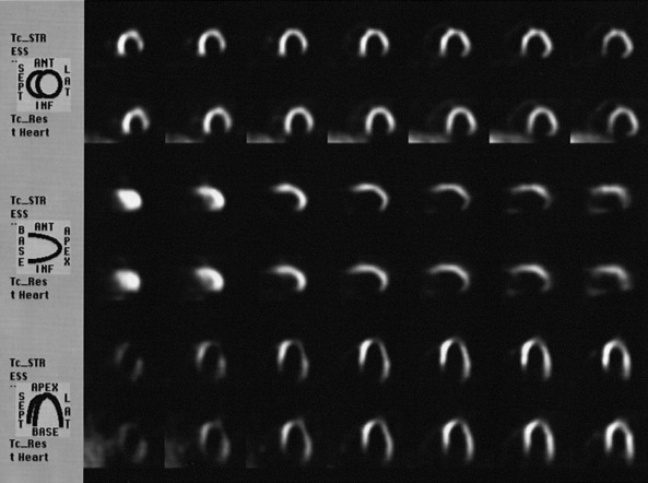
The data can be reformatted into planes oblique to the original transverse planes. This is particularly useful in cardiac imaging, in which the long axis of the heart does not coincide with any of the three major axes of the reconstructed data. It is desirable to reorient the data to obtain images that are perpendicular and parallel to the long axis of the left ventricle, which can be readily accomplished from the original volume data set. The computer operator defines the geometry of the long axis of the heart, and the data are reformatted to create cardiac long-axis and short-axis planes oblique to the transaxial slices ( Fig. 3.7 ). The optimum angulation is highly variable across patients.