TP  =  test positive in diseased subjects

FP  =  test positive in nondiseased subjects

FN  =  test negative in diseased subjects

TN  =  test negative in nondiseased subjects

T+   =  abnormal test results

T-    =  normal test results

D+   =  diseased subjects

D-   =  nondiseased subjects

STATISTICS

Incidence   =  number of diseased people per 100,000 population annually

Prevalence   =  number of existing cases per 100,000 population at a target date

Frequency   =  number of times an event occurred; often graphically represented in histograms

Mortality   =  number of deaths per 100,000 population annually

Fatality   =  number of deaths per number of diseased

Sensitivity

=  ability to detect disease

=  probability of having an abnormal test given disease

=  number of correct positive tests / number with disease

=  true positive ratio = TP / (TP + FN) = TP / D+

•  D+ column in decision matrix

◊  Independent of prevalence

Specificity

=  ability to identify absence of disease

=  probability of having a negative test given no disease

=  number of correct negative tests / number without disease

=  true negative ratio = TN / (TN + FP) = TN / D-

•  D- column in decision matrix

◊  Independent of prevalence

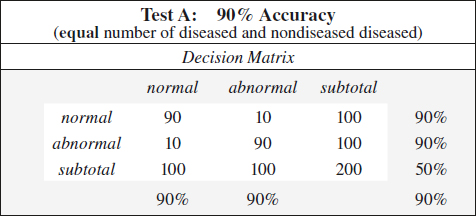
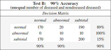
Accuracy

=  number of correct results in all tests

=  number of correct tests / total number of tests

=  (TP + TN) / (TP + TN + FP + FN) = (TP + TN) / total

◊  Depends much on the proportion of diseased + nondiseased subjects in studied population

◊  Not valuable for comparison of tests

Example:   same test accuracy of 90% for two tests A and B

Positive Predictive Value

=  positive test accuracy

=  likelihood that a positive test result identifies disease

=  number of correct positive tests / number of positive tests

=  TP / (TP + FP) = TP / T+

•  T+ row in decision matrix

◊  Dependent on prevalence

◊  PPV ↑ with ↑ prevalence for given sensitivity + specificity

◊  PPV ↑ with ↑ specificity for given prevalence

Negative Predictive Value

=  negative test accuracy

=  likelihood that a negative test result identifies absence of disease

=  number of correct negative tests / number of negative tests

=  TN / (TN + FN) = TN / T-

•  T- row in decision matrix

◊  Dependent on prevalence

◊  NPV ↑ with ↑ prevalence for given sensitivity + specificity

◊  NPV ↑ with ↑ sensitivity for given prevalence

False-positive Ratio

=  proportion of nondiseased patients with abnormal test result

•  D- column in decision matrix

=  FP / (FP + TN) = FP / D-

=  1 – specificity = (TN + FP – TN) / (TN + FP)

False-negative Ratio

=  proportion of diseased patients with a normal test result

•  D+ column in decision matrix

=  FN / (TP + FN) = FN / D+

=  1 – sensitivity = (TP + FN – TP) / (TP + FN)

Disease Prevalence

=  proportion of diseased subjects to total population

=  (TP + FN) / (TP + TN + FP + FN) = D+ / total

◊  Affects predictive values + accuracy of a test result

Example:

Test A, C, D:   90% sensitivity + 90% specificity

Bayes Theorem

=  the predictive accuracy of any test outcome that is less than a perfect diagnostic test is influenced by

(a)  pretest likelihood of disease

(b)  criteria used to define a test result

Receiver Operating Characteristics (ROC)

=  degree of discrimination between diseased + nondiseased patients using varying diagnostic criteria instead of a single value for the TP + TN fraction

=  curvilinear graph generated by plotting TP ratio as a function of FP ratio for a number of different diagnostic criteria (ranging from definitely normal to definitely abnormal)

Y-axis:   true-positive ratio = sensitivity

X-axis:   false-positive ratio = 1 – specificity; reversing the values on the X-axis results in an identical “sensitivity-specificity curve”

Use:     variations in diagnostic criteria → reported as a continuum of responses → ranging from definitely abnormal to equivocal to definitely normal ← based on subjectivity + bias of individual radiologists

◊  A minimum of 4–5 data points of diagnostic criteria are needed!

Difficulty:   subjective evaluation of image features; subjective diagnostic interpretation; data must be ordinal (= discrete rating scale from definitely negative to definitely positive)

Interpretation:

◊  ↑ in sensitivity leads to ↓ in specificity!

◊  ↑ in specificity leads to ↓ in sensitivity!

◊  Most sensitive point is the point with the highest TP ratio

→  equivalent to “overreading” by using less stringent diagnostic criteria (all findings read as abnormal)

◊  Most specific point is the point with the lowest FP ratio

→  equivalent to “underreading” by using more strict diagnostic criteria (all findings read as normal)

◊  Does not consider disease prevalence in the population

Related posts:

and Soft-Tissue Disorders Anatomy and Mammographic Technique AND GYNECOLOGY and Function of Lung BREAST of the Nervous System

Stay updated, free articles. Join our Telegram channel

Join