Abstract
In vivo magnetic resonance imaging of the spinal cord is challenging due to susceptibility variations between various tissue types, air in the lungs and trachea, and in some cases surgical implants that significantly distort the applied magnetic field. These field inhomogeneities create off-resonance induced artifacts in the images, such as signal dropouts and pileups, geometric distortions, and incomplete fat suppression. Bulk physiologic motion from cardiac and respiratory cycles, cerebrospinal fluid pulsation, as well as breathing and swallowing further cause temporal variations of these field inhomogeneities. Moreover, the anatomy of the spine requires a relatively large field of view (FOV), especially in the sagittal imaging plane, while the small cross-sectional size of the spinal cord mandates high-spatial-resolution images. The resulting long readout duration, especially that of echo planar imaging (EPI), further exacerbates the artifacts. This chapter reviews susceptibility artifacts, their impact on EPI of the spinal cord, and methods to limit these artifacts. Acquisition-based methods include multishot imaging, parallel acquisitions, reduced-FOV methods, and non-EPI techniques. Reconstruction-based methods involve distortion correction, phase correction, and other advanced techniques.
Keywords
Distortion, Echo-planar imaging (EPI), Field inhomogeneity, Off-resonance, Signal dropout, Signal pileup, Susceptibility artifacts
2.3.1
Introduction: Sources of Susceptibility Artifacts
The uniformity of the B 0 main field in magnetic resonance imaging (MRI) is critical for artifact-free image formation. MRI scanners are manufactured with a stringent requirement of less than one part-per-million (ppm) a
a In MRI, the variations in B 0 field or the differences in resonant frequencies are so small that they are expressed in “parts per million”, or ppm. For example, 1 ppm inhomogeneity at 1.5 T corresponds to a 1.5 μT variation in the B 0 field. This field variation would in turn result in a 63.87 Hz off-resonance (i.e., one-millionth of the center frequency of f 0 = 63.87 MHz at 1.5 T).
variation in the B 0 field. However, this 1 ppm theoretical homogeneity easily gets distorted once a subject is placed inside the MRI scanner, mainly due to a 9 ppm magnetic susceptibility difference between air and tissue. The presence of any surgical implants further exacerbates the problem, as different tissue types, air, and metal all interact with and distort the applied magnetic field differently. This interaction is quantified by what is called the magnetic susceptibility of a matter.The susceptibility variations in tissue on a microscopic scale are in fact the source of many useful contrast mechanisms in MRI, such as blood oxygenation level-dependent (BOLD) functional MRI (fMRI) and diagnosis of cerebral hemorrhage. However, a macroscopic susceptibility variation leads to a global field inhomogeneity, which in turn creates off-resonance induced artifacts in the images. These artifacts manifest as faster T 2 ∗ decay, signal dropouts and pileups, geometric distortions, and incomplete fat suppression. High-field MRI scans especially suffer from susceptibility artifacts, as the absolute size of the field perturbations increases linearly with B 0 field strength. For example, the 9 ppm susceptibility difference between air and tissue corresponds to a 575 Hz field variation at 1.5 T, while it is doubled to a 1150 Hz variation at 3 T. While a global frequency shift can be easily dealt with by adjusting the center frequency, it is the local field inhomogeneity that perturbs the imaging process.
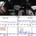
In vivo MRI of the spinal cord is especially challenging due to susceptibility variations between various tissue types (e.g., vertebrae, muscle, CSF, gray and white matter, fat, air in the lungs and trachea, bowel gas, and surgical implants) that significantly distort the applied magnetic field. As shown by the B 0 field maps of the spine ( Figure 2.3.1 ), the air in the lungs and nasal cavities as well as the curvature in the neck significantly distort the field around the spinal cord. Furthermore, susceptibility differences between vertebral spinous processes and connective tissue create local field inhomogeneities along the spinal cord itself, as seen in Figure 2.3.1 (B). Bulk physiologic motion from cardiac and respiratory cycles, CSF pulsation, as well as breathing and swallowing further cause temporal variations of these field inhomogeneities.

This chapter gives an overview of susceptibility artifacts and how they manifest in EPI images of the spinal cord. Methods to alleviate these artifacts will be outlined. Please note that while this chapter mostly presents examples of susceptibility artifacts on sagittal images, axial and coronal orientations are equally affected.
2.3.2
Artifacts in EPI of the Spinal Cord
Single-shot echo planar imaging (ss-EPI) remains the most frequently used technique for most of the quantitative imaging methods, because it acquires the whole of k -space after a single excitation. This fast imaging capability is especially critical for methods that are sensitive to subject motion (e.g., diffusion-weighted imaging (DWI)) or for methods that require a high temporal resolution (e.g., fMRI).
Although ss-EPI performs relatively well in the brain, the anatomy of the spine as well as the abundance of susceptibility variations make it particularly difficult to produce high-quality ss-EPI images of the spinal cord. The long and narrow anatomy of the spine requires a large field of view (FOV) in the superior-inferior (S/I) direction, and the small cross-sectional size of the spinal cord mandates high-spatial-resolution images. Even in the axial imaging plane, where the spinal cord presents a small region of interest (ROI), the rest of the body dictates a large FOV. Covering a large FOV with high resolution requires long readout durations in EPI, which in turn result in distortions and severe blurring of the images along the phase-encoding (PE) direction. In addition, the long interval between subsequent k -space lines (i.e., echo spacing) causes significant image distortions due to off-resonance effects.
The location-dependent geometric distortion in an EPI image can be expressed as:
d PE ( r ) = Δ f ( r ) T ESP FOV PE N int R .

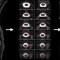
ss-EPI images also exhibit a substantial water–fat misalignment, as the frequency term in Eqn (2.3.1) also applies to chemical shifts. For example, for the aforementioned imaging parameters, the fat image would experience a 4 cm shift in the PE direction with respect to the water image (assuming a chemical shift of 3.5 ppm, i.e., 440 Hz at 3 T). Hence, ss-EPI mandates proper shimming of the ROI, as well as a robust fat suppression or spectrally selective excitation. These fat suppression schemes usually take advantage of the chemical shift (i.e., differences in resonant frequencies) between fat and water. Unfortunately, susceptibility variations around the spine can distort the field homogeneity to such an extent that effective fat suppression is often an issue. For example, a local 440 Hz susceptibility-induced off-resonance at 3 T would cause the water signal to be suppressed, instead of the fat signal. Figure 2.3.2 (B) demonstrates this phenomenon, where the susceptibility variations around the cervical spine resulted in an incomplete fat suppression (white arrow) and a signal dropout (red arrow).
The position dependency of susceptibility effects causes different regions in the FOV to experience different levels of displacement, further complicating the problem. This nonrigid distortion is typically observed as signal pileups or dropouts in an EPI image. The cervicothoracic junction in Figure 2.3.2 (C) shows one such case, where the signals from the spinal cord and the CSF are piled up, while the neighboring pixels (where CSF was supposed to be) are left devoid of signal (yellow arrow). A less severe manifestation of this susceptibility artifact is the comb-like appearance of the spinal cord in Figure 2.3.2 (C), which is caused by the local field inhomogeneities along the spinal cord (see Figure 2.3.1 (B)).
2.3.3
Methods to Reduce Susceptibility Artifacts
There are various approaches that can be used to reduce susceptibility artifacts for spinal cord imaging; unfortunately, many of these methods have only been demonstrated in the research arena and are not available on clinical scanners. These approaches target one (or more) of the variables in Eqn (2.3.1) , which can be rewritten as:
d PE ( r ) = Δ f ( r ) S k
S k = Δ k PE Δ t PE = N int R FOV PE T ESP
Related posts:


Stay updated, free articles. Join our Telegram channel

Full access? Get Clinical Tree


